
In this post, I talk about the current state of memristor modeling after having rolled up my sleeves for the last several weeks, getting my hand dirty with as many open source circuit simulators as possible, and simulating memristors using various techniques and approaches. I’ve gained a lot of insight into the current state of the art of memristor modeling that I thought would be worth documenting.
“Hacked” SPICE Subcircuit Memristor Models
Around 2008, the first memristor models designed for SPICE started showing up. A paper by Biolek et al. showed how to implement a memristor model in SPICE as a .subckt. I call this a “hacked” model because in order to implement it you are constrained in using only existing SPICE elements such as resistors, capacitors, and various specialized voltage and current sources, hacking together a model from these pieces. In a previous post of mine The Joglekar Resistance Switch Memristor Model in LTSpice, I explain in great detail how it works, and I demonstrate a working model and simulation in LTSpice.
The following is the SPICE model from the LTSpice link above:
|
1 2 3 4 5 6 7 8 9 10 11 12 13 14 15 16 17 18 19 20 21 22 23 24 25 26 27 28 29 30 31 32 33 34 35 36 37 38 39 40 41 42 43 44 45 46 47 48 49 50 51 52 53 54 55 56 |
*********************************************** * HP Memristor SPICE Model * For Transient Analysis only * created by Zdenek and Dalibor Biolek *********************************************** * Ron, Roff - Resistance in ON / OFF States * * Rinit - Resistance at T=0 * * D - Width of the thin film * * uv - Migration coefficient * * p - Parameter of the WINDOW-function for * modeling nonlinear boundary conditions * * x - W/D Ratio, W is the actual width * of the doped area (from 0 to D) * *********************************************** .SUBCKT memristor plus minus PARAMS: + Ron=100 Roff=16K Rinit=11K D=10N uv=10F p=1 *********************************************** * DIFFERENTIAL EQUATION MODELING * *********************************************** Gx 0 x value={I(Emem)*uv*Ron/D**2*f(V(x),p)} Cx x 0 1 IC={(Roff-Rinit)/(Roff-Ron)} Raux x 0 1000000 *********************************************** * RESISTIVE PORT OF THE MEMRISTOR * *********************************************** Emem plus aux value={-I(Emem)*V(x)*(Roff-Ron)} Roff aux minus {Roff} *********************************************** * FLUX COMPUTATION * *********************************************** Eflux flux 0 value={SDT(V(plus,minus))} *********************************************** * CHARGE COMPUTATION * *********************************************** Echarge charge 0 value={SDT(I(Emem))} *********************************************** * WINDOW FUNCTIONS * FOR NONLINEAR DRIFT MODELING * *********************************************** * window function, according to Joglekar .func f(x,p)={1-(2*x-1)**(2*p)} .ENDS memristor |
While the simulation was successful, there are some disadvantages of this type of model:
- The model is unintuitive and hard to understand because it is hacked together.
- It only works for transient analysis, not DC sweeps.
- It suffers from convergence issues at initial conditions and edge cases (See Note)
- Netlist size grows quickly for large circuits with memristors.
Note: Simulating this same mode in NGSpice and JSpice (our internal Java-based SPICE simulator) yielded convergence issues at the first time step. It did however work just fine in Xyce.
Ill-posed Models
In another class of models, the memristor is usually defined in a more flexible and less hacked manner in a language such as Verilog-A, MATLAB or ModSPEC. In such simulation environments, you are given a blank slate to formulate your model using the language’s full API and methods. Inside your model implementation, you are given access to the global voltage drop across the device and from there you define the current. You are also given the simulation time, and you can use this to calculate how long a certain voltage was applied since the last time-step–important in modeling memristors given their memory/flux behavior.
In order to demonstrate this, here is the Joglekar model again, but implemented in Verilog-A and simulated in Xyce. For anyone interested in running this yourself you may want to check out Build Xyce from Source for ADMS Verilog-A Model Integration.
Joglekar Resistance Switch Model in Verilog-A (Xyce Flavor) memristor.va
The following code can be found on the memristor-models-4-all project.
|
1 2 3 4 5 6 7 8 9 10 11 12 13 14 15 16 17 18 19 20 21 22 23 24 25 26 27 28 29 30 31 32 33 34 35 36 37 38 39 40 41 42 43 44 45 46 47 48 49 50 51 52 53 54 55 56 57 58 59 60 61 62 63 64 65 66 67 68 69 70 71 72 73 74 75 76 77 78 79 80 81 82 83 84 85 86 |
`include "disciplines.vams" `include "constants.vams" `define X_BORDER_BUMP 10e-18 `define attr(txt) (*txt*) module memristor1 (p,n); inout p,n; electrical p,n; parameter real Roff=16000 from (0:inf) `attr(info="Roff" type="instance"); parameter real Ron=100 from (0:inf) `attr(info="Ron" type="instance"); parameter real Rinit=11000 from (0:inf) `attr(info="Rinit" type="instance"); parameter real D=10n from (0:inf) `attr(info="D" type="instance"); parameter real uv=10e-15 from (0:inf) `attr(info="uv" type="instance"); parameter real p_coeff=1.0 from (0:inf) `attr(info="p_coeff" type="instance"); // local variables that should persist over time steps real w_last; real time_last; // local variables that hold temporary values real G; real window_function; real w; real dw; real R; real direction; real current; real time; real time_delta; analog begin @(initial_instance) begin w_last = ((Roff - Rinit) / (Roff - Ron)) * D; time_last = 0; end // calculate conductance G = 1 / (Ron * w_last / D + Roff * (1 - w_last / D)); current = G * V(p,n); direction = 0; if (current > 0) begin if(w_last<=0) begin direction=1; end end else begin if(w_last>=D) begin direction=-1; end end time = $realtime; time_delta = time - time_last; window_function = (1.0 - (pow(2 * w_last / D - 1, 2 * p_coeff))); dw = uv * Ron / D * current * window_function * time_delta; w = w_last + dw + direction * `X_BORDER_BUMP; if(w >= D) begin w = D; end if(w <= 0) begin w = 0; end // calculate conductance G = 1 / (Ron * w / D + Roff * (1 - w / D)); // set the current I(p,n) <+ -1.0*G*V(p,n); // persist variables w_last = w; time_last = time; end endmodule |
Simulation File (Xyce) memristor_sim.cir
|
1 2 3 4 5 6 7 8 9 10 11 12 13 |
* Voltage Sources V1 1 0 SIN(0V 1.2V 1Hz) * Memristors YMEMRISTOR1 M1 1 0 * Analysis Command .TRAN 1ms 1s * Output .PRINT TRAN V(1) I(V1) .END |
Simulation Commands
|
1 2 3 4 5 6 |
cd .../Linear\ Resistance\ Switch/Verilog-A buildxyceplugin -o memristor *.va /usr/local/lib Xyce -plugin /usr/local/lib/memristor.so memristor_sim.cir gnuplot plot '.../Linear_Resistance_Switch/Verilog-A/memristor_sim.cir.prn' using 3:4 with lines title "I-V" |
Result
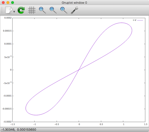
Xyce Joglekar Memristor Model
While the simulation was successful, there are some disadvantages of this type of model:
- It only works for transient analysis, not DC sweeps
- Need to calculate
dtastime_deltain order to perform an integration - Must declare a
realas the general variable to hold the state of the device - Explicitly guarding against non-physical conditions for
w
In fact, these issues are only the tip of the iceberg. If you understand the internal workings of the simulator, there are more issues at play here.
Well-posed Models
In May, 2016, Wang and Roychowdhury published an excellent paper titled Well-Posed Models of Memristive Devices, in which they plainly list out all of the problems with the current approaches and implementations of memristor models. In their words:
In spite of seemingly significant efforts to devise memristor models, every model we are aware of in the literature [25–30] suffers from one or more of the above-mentioned types of ill-posedness.
The types are:
Common ill-posedness mechanisms in models include division-by-zero errors, often due to expressions like 1/(x−a), which become unbounded (and feature a “doubly infinite” jump) at x=a; the use of log(), 1/(x−a) or sqrt() without ensuring that their arguments are always positive, regardless of bias; the fundamental misconception that non-real (i.e., complex) numbers or infinity are legal values for device models (they are not!); and “sharp”/“pointy” functions like |x|, whose derivatives are not continuous. Another key aspect of well-posedness is that the model’s equations must produce mathematically valid outputs for any mathematically valid input to the device. Possibly the most basic kind of input is one that is constant (“DC”) for all time. DC solutions (“operating points”) are fundamental in circuit design; they are typically the kind of solution a designer seeks first of all, and are used as starting points for other analyses like transient, small signal AC, etc. If a model’s equations do not produce valid DC outputs given DC inputs, it fails a very fundamental well-posedness requirement. For example, the equation d/dt o(t) = i(t) is ill posed, since no DC (constant) solution for the output o(t) is possible if the input i(t) is any non-zero constant. Such ill posedness is typically indicative of some fundamental physical principle being violated; for example, in the case of d/dt o(t) = i(t), the system is not strictly stable [24]. Indeed, a well-posed model that is properly written and implemented should work consistently in every analysis (including DC, transient, AC, etc.).
They do a good job in explaining the problems in detail, while also proposing a better way to approach memristor model development at a fundamental level, which I won’t repeat here. Rather, I take their Verilog-A/Xyce example for a generic memristor directly from their paper, add some necessary tweaks, and show the results.
Generic Model in Verilog-A (Xyce Flavor) hys.va
The following code can be found on the memristor-models-4-all project.
|
1 2 3 4 5 6 7 8 9 10 11 12 13 14 15 16 17 18 19 20 21 22 23 |
// A device with hysteresis `include "disciplines.vams" `define attr(txt) (*txt*) module hys(p, n); inout p, n; electrical p, n, ns; parameter real R = 1e3 from (0:inf) `attr(info="R" type="instance"); parameter real k = 1 from (0:inf) `attr(info="k" type="instance"); parameter real tau = 1e-5 from (0:inf) `attr(info="tau" type="instance"); real s; analog begin s = V(ns, n); I(p, n) <+ V(p, n)/R * (1+tanh(k*s)); I(ns, n) <+ V(p, n) - pow(s, 3) + s; I(ns, n) <+ ddt(-tau*s); end endmodule |
Forward DC Sweep test_hys_forward.cir
|
1 2 3 4 5 6 7 8 9 |
* test hys.va in DC forward V1 1 0 1 sin(0 0.7 1k) Yhys H1 1 0 * DC analysis .dc V1 -1 1 0.01 .print dc V(1) I(V1) N(Yhys!H1_ns) |
Reverse DC Sweep test_hys_reverse.cir
|
1 2 3 4 5 6 7 8 9 |
* test hys.va in DC reverse V1 1 0 1 sin(0 0.7 1k) Yhys H1 0 1 * DC analysis .dc V1 -1 1 0.01 .print dc V(1) I(V1) N(Yhys!H1_ns) |
Transient test_hys_transient.cir
|
1 2 3 4 5 6 7 8 9 |
* test hys.va in transient V1 1 0 1 sin(0 0.7 1k) Yhys H1 1 0 * transient simulation .tran 1u 2m .print tran V(1) I(V1) N(Yhys!H1_ns) |
Simulation Commands
|
1 2 3 4 5 6 7 8 9 |
cd .../memristor-models-4-all/Generic/Verilog-A buildxyceplugin -o hys *.va /usr/local/lib Xyce -plugin /usr/local/lib/hys.so test_hys_forward.cir Xyce -plugin /usr/local/lib/hys.so test_hys_reverse.cir Xyce -plugin /usr/local/lib/hys.so test_hys_transient.cir gnuplot plot '.../memristor-models-4-all/Generic/Verilog-A/test_hys_forward.cir.prn' using 2:3 with lines title "forward DC Sweep", '.../memristor-models-4-all/Generic/Verilog-A/test_hys_reverse.cir.prn' using 2:3 with lines title "reverse DC Sweep", '.../memristor-models-4-all/Generic/Verilog-A/test_hys_transient.cir.prn' using 3:4 with lines title "Transient" |
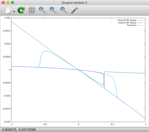
Xyce Well-posed Memristor Model
The currents are negative, and the reverse DC sweep X-axis and Y-Axis should be flipped, but the results are the same as shown in the above referenced paper by Wang et al. You can see here that the results are valid for both transient and DC analysis!
The strategy implemented in the above model is explained as:
To circumvent these issues and write a robust Verilog-A model for
hys_examplethat should work consistently in all simulators and all simulation algorithms, we model state variablesas a voltage. We declare an internal branch, whose voltage representss. One end of the branch is an internal node that doesn’t connect to any other branches. In this way, by contributingV − s^3 + sandddt(-tau * s)both to this same branch, the KCL at the internal node will enforce the implicit differential. Declaringsas a voltage is not the only way to modelhys_examplein Verilog-A. Depending on the physical nature ofs, one can also use Verilog-A’s multiphysics support and model it as a mechanical property, such as a position from the kinematic discipline. This may be closer to the actual meaning ofsfor MIM-structured RAM devices. Alternatively, we can also use the property for potential from the thermal or magnetic discipline. One can also switch potential and flow by definingsas a flow instead. These alternatives may make the model look more physical, but they do not make a difference mathematically, except from the scale of tolerances in each discipline, which we will discuss in more detail in Sec. IV-C. The essence of our approach is to recognize that state variable s is a circuit unknown, and thus should be modeled as a potential or flow in Verilog-A, for the consistent support from different simulators in various circuit analyses.
Again, you should read the full paper. Hats off to Wang and Roychowdhury, as this is a push in the right direction that the memristor modeling community needs.
Homotopy Analysis
Continuation algorithms, also known as homotopy algorithms are normally used to sweep the magnitudes of independent voltage and current sources when a DC operating point calculation fails to converge. Homotopy analysis can track the DC solution curve in the state space. Xyce will apply source stepping automatically during the DC operating point calculation if both the standard Newton’s method and GMIN stepping fail. So, normally, this technique of manually forcing stepping of a single source is unnecessary. But we can actually use it to take a look at some of the parameters in our memristor model as pointed out in the Wang and Roychowdhury paper. For completeness, I demonstrate this as well. As you will see, the results show that as all DC points, the model is continuous.
From the Xyce 6.6 User Manual:
Another basic type of continuation in Xyce is accessed by setting
.options nonlin continuation=1. This allows the user to sweep existing device parameters (models and instances), as well as a few reserved artificial parameter cases. The most obvious natural parameter to use is the magnitude(s) of independent voltage or current sources, the choice of which is equivalent to “source stepping” in SPICE. Section 8.2 provides a Xyce source-stepping example. For some circuits (as in the aforementioned Schmidt trigger), source stepping leads to turning points in the continuation.
Homotopy test_hys_homotopy.cir
|
1 2 3 4 5 6 7 8 9 10 11 12 13 14 15 16 |
* test hys.va in Homotopy V1 1 0 1 sin(0 0.7 1k) Yhys H1 1 0 * homotopy analysis .dc V1 .7 .7 1 .print homotopy V(1) I(V1) N(Yhys!H1_ns) .options nonlin continuation=1 .options loca stepper=ARC + predictor=1 stepcontrol=1 + conparam=V1:DCV0 + initialvalue=-1.0 minvalue=-1.0 maxvalue=1.0 + initialstepsize=0.01 minstepsize=1.0e-8 maxstepsize=0.1 + aggressiveness=0.1 |
Simulation Commands
|
1 2 3 4 |
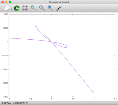
Xyce -plugin /usr/local/lib/hys.so test_hys_homotopy.cir plot '.../memristor-models-4-all/Generic/Verilog-A/test_hys_homotopy.cir.HOMOTOPY.prn' using 3:4 with lines title "I" plot '.../memristor-models-4-all/Generic/Verilog-A/test_hys_homotopy.cir.HOMOTOPY.prn' using 3:5 with lines title "S" |
Results
| Current | State |
|---|---|
 |
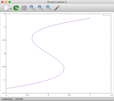 |
Indeed the DC analysis forms a smooth curve in the state space. The corresponding curve in current consists of all the unstable solutions in the i–v relationship (wherever the slope of S is negative).
This curve was previously missing in DC and transient sweep results, and now displayed by the homotopy analysis. These results from homotopy analysis provide us with important insights into the model. They reveal that there is a single smooth and continuous DC solution curve in the state space, which is an indicator of the well-posedness of the model. They also illustrate that it is the folding in the smooth DC solution curve that has created the discontinuities in DC sweep results. These insights are important for the proper modelling of hysteresis. Moreover, the top view explains the use of internal state s for modeling hysteresis from another angle. Without the internal state, it would be difficult if not impossible to write a single equation describing the i–v relationship. With the help of
s, we can easily choose two simple model equations, and the complex i–v relationship forms naturally.
Further Resources
- Knowm Memristors
- The Generalized Metastable Switch Memristor Model
- The Problem is Not HP’s Memristor–It’s How They Want To Use It
- The Joglekar Resistance Switch Memristor Model in LTSpice
- Build Xyce from Source for ADMS Verilog-A Model Integration
- The Pershin Voltage Threshold Memristor Model in NGSpice
- memristor-models-4-all Project on Github


3 Comments
Paritosh Sahu
Hello Tim, This is great work you all are doing. I am a student researching on RRAM myself. I have read the same paper recently, and it is excellent. I have thought of implementing the models on real fabricated samples and see how they stack up against the experimentally obtained curves. Hope you could help me out if i get stuck in between. Cheers!
syed abdul rahim
whenever am excuting verilo a code of memristor in cadence am getting the error like “extract failed for cell view”
can any body clarify this problem?
Lokesh
kindly contact me i want to talk