The Joglekar Resistance Switch Memristor Model in LTSpice

Sign up for our newsletter for progress updates, product announcements and Knowm news.

Close-up of one of the 4X4X8 crossbar die in a crossbar module

In 2009, Biolek et al. published a paper showing an idealized memristor model for a newly publicized memristor created at HP labs. The paper can be downloaded here. The model is referred to in a fews ways: “The Ideal Memristor”, “The nonlinear Dopant Drift” or “The Resistance Switch”. For anyone starting out simulating memristors in SPICE, this is probably the first thing you will try before getting into more complicated (and accurate) models. So after reading that paper and understanding the basic idea, the next step is to fire up SPICE and repeat the results in the paper. This blog post is about taking the model from the paper and getting the classic memristor hysteresis I-V plot in LTSpice. These concepts can be adapted for different SPICE simulators and models.

Model Overview

The model is described quite well in the above referenced paper, but lets review the most critical pieces needed to understand how SPICE implementation works. In the model, there is a window function:

Which looks like this:

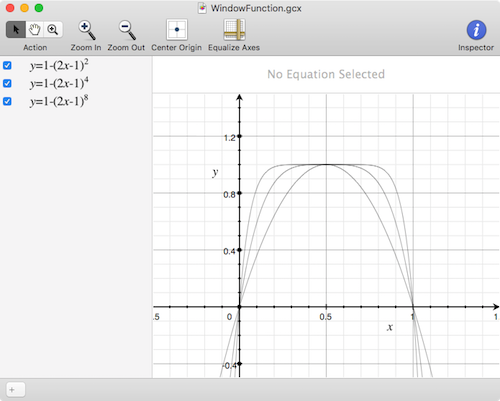
Joglekar dopant drift window function

If you plot the integral of this function between 0 and 1, you get this:

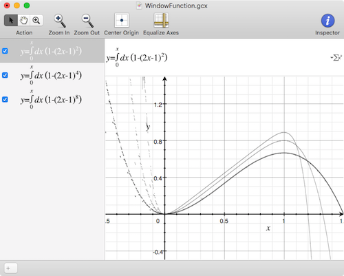
Joglekar dopant drift window function integral

In this model the integral of the window function represents the state x, between 0 and 1, and is used to dynamically change a delta R value. delta R is Roff - Ron, and when in series with Roff (and given a minus sign) defines the memristor resistance. Conveniently a current source in series with a 1F capacitor and a resistor creates an integrator circuit, where the voltage on node x represents the integral.

Download and Install LTSpice

If you haven’t already, you need to download and install LTSpice. I’m using a Mac so I installed it via homebrew: brew cask install ltspice.

Note where the application installed, as we need to add some files in appropriate places. In my case the root directory is at ~/Library/Application\ Support/LTspice/.

Add the Memristor Subcircuit and Symbol Files

The following code can be found on the memristor-models-4-all project.

Create a file called memristor.sub and save it in .../LTSpice/lib/sub. Put the following text in it:

Note that I changed the p variable to 1. With p=1 the results will match what’s in the paper.

Create a file called memristor.asy and save it in .../LTSpice/lib/sym. Put the following text in it:

This file defines a new graphical symbol for the memristor.

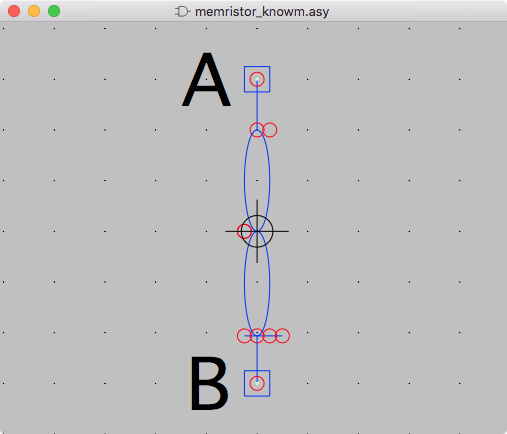
ltspice knowm memristor symbol

Add the Simulation File

Create a file called memristor_sim.asc and save it in somewhere in your normal documents directory such as ~/Documents/LTSpice. This is the directory created by LTSpice on my machine and contains some example simulation files already.

Open the Simulation File

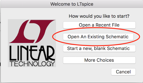
open schematic ltspice

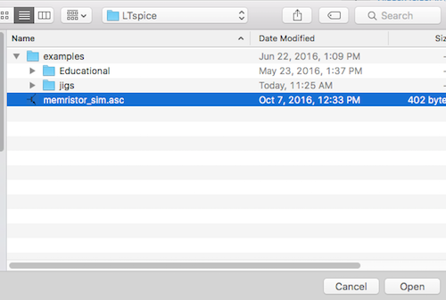
memristor sim ltspice

Set up a Few Things before Running SPICE Simulation

In the schematic window, click the tools button.

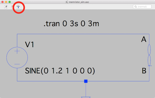
ltspice memristor sim schematic

Make sure the following options are checked:

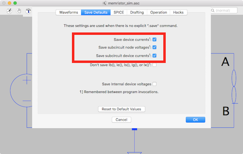
ltspice schematic tools

Run Simulation and View Results

After clicking the run button, a blank plot will pop up. You need to select all the correct traces by right-clicking and selecting add Traces. Just select Ix(Memristor:A).

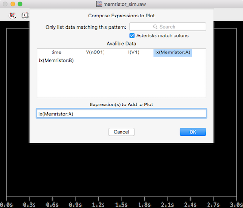
ltspice memristor current

Next, on the plot, click on the X axis and change time to V(n001).

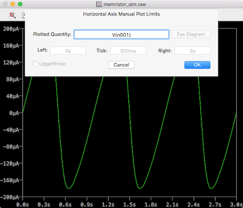
ltspice memristor horizontal axis

Now you should see the I-V pinched hysteresis plot.

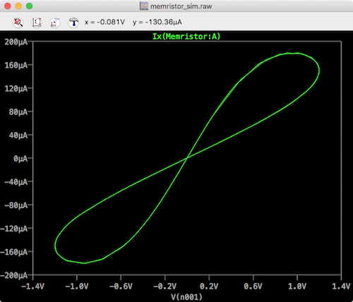
ltspice memristor hysteresis

Next you can clear the plot pane and add several other simulation results as a function of time:

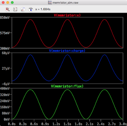
ltspice memristor time

Here we see from top down:

1. The state variable x. Note it’s between 0 and 1
2. The charge through the device
3. The flux through the device

Conclusion

While we wouldn’t claim that this memristor model is an ideal model for Knowm’s memristors (or any memristor really), understanding how the mathematics of the model works as well as the mechanics of the SPICE simulation and the memristor subcircuit is an important step towards developing better models. Be sure to stay tuned by signing up for our newsletter and/or subscribing to our RSS feed to get the latest information about our memristor modeling progress. In the future, we will be blogging about other SPICE tools, our Metastable Switch memristor model, and other memristor modeling advancements!

Further Resources

• Knowm Memristors
• The Generalized Metastable Switch Memristor Model
• The Problem is Not HP’s Memristor–It’s How They Want To Use It
• memristor-models-4-all Project on Github
• The Pershin Voltage Threshold Memristor Model in NGSpice
• Build Xyce from Source for ADMS Verilog-A Model Integration
• Well-posed Memristor Modeling with Xyce and Verilog-A