The Mean Metastable Switch Memristor Model in Xyce

In a previous post titled Native Memristor Device Development in Xyce, I showed how to create the Joglekar memristor model natively in Xyce, by first cloning an existing Yakopcic device model followed by implementing the Joglekar’s dX/dt behavior. In this post, I show how we first modified our current memristor model – the Metastable Switch Model – in order to fit into the Xyce si\mulator’s constraints followed by the code showing the implementation. Full source code for the model can be found at the memristor-models-4-all Project on Github.

Memristor Modeling in Xyce

In order to be more in-line with conventional memristor models, and to tie into the “Xyce Way”, we needed to adapt our current MSS model in 4 ways:

Define on and off conductances as resistances
Define the two main resistance levels as On and Off rather than A and B
Define the main state of the device as X [0,1], rather than N_off. It’s the same but it’s scaled to one and is continuous.
Define the state, X, in terms of $dX/dt$ .

Defining On and Off aren’t strictly necessary for Xyce, but \much easier for everyone else to understand the model at first sight, as it’s become the standard convention in memristor modeling. For a different reference to see how other groups define $dX/dt$ , see the Yakopcic Model, equation 7.

Model Conversion to dX/dt

Parameters

First off, here is a summary of the model parameters. Note that for now, I removed the two oppositely connected Schottky diodes in parallel with the collection of metastable switches.

Name	Units	Description
ROFF	Ohm	Off resistance
RON	Ohm	On resistance
VOFF	Volts	Threshold voltage to turn device off
VON	Volts	Threshold voltage to turn device on
\tau	Seconds	Time constant

Note that $T$ (temperature) is also a parameter hidden in $\beta = \frac{q}{{kT}} = {({V_{T}})^{-1}}$ .

Starting with what we already had, the change in the number of switches, scaled between 0 and 1, $dX$ is:

$dX = \frac{N_{OFF \rightarrow ON} - N_{ON \rightarrow OFF} }{N}$

If the probabilities $P_{OFF \rightarrow ON}$ and $P_{ON \rightarrow OFF}$ are defined as:

$P_{OFF \rightarrow ON} = \alpha \frac{1}{{1 + {e^{ \beta \left( {V - {V_{ON}}} \right)}}}}$ $P_{ON \rightarrow OFF} = \alpha \left(1 - \left(\frac{1}{{1 + {e^{ \beta \left( {V + {V_{OFF}}} \right)}}}}\right)\right)$

and we define a function $N'$ as a Gaussian sample, such as the Box-\muller Transform:

$N'\left( {\mu ,{\sigma ^2}} \right) = Some algo returning a random sample$

, then

$dX = \frac{N'\left( {\mu_{OFF} ,{\sigma_{OFF \rightarrow ON} ^2}} \right) - N'\left( {\mu_{ON} ,{\sigma_{ON \rightarrow OFF} ^2}} \right) }{N}$

. If $\mu_{OFF} = N-X N$ , $\mu_{ON} = X N$ , $\sigma_{OFF \rightarrow ON} = N P_{ON \rightarrow OFF}(1-P_{OFF \rightarrow ON})$ , $\sigma_{ON \rightarrow OFF} = N P_{ON \rightarrow OFF}(1-P_{ON \rightarrow OFF})$

, then

$dX = \frac{N'\left( {N-X N ,{N P_{OFF \rightarrow ON}(1-P_{OFF \rightarrow ON}) ^2}} \right) - N'\left( {X N ,{N P_{ON \rightarrow OFF}(1-P_{ON \rightarrow OFF} ^2}} \right) }{N}$

. Therefore plugging everything in (really ugly!), also setting $\alpha = \frac{dT}{\tau}$ :

$dX = \frac{N'\left( {N-X N ,{N \frac{dT}{\tau} \frac{1}{{1 + {e^{ \beta \left( {V - {V_{ON}}} \right)}}}}(1-\frac{dT}{\tau} \frac{1}{{1 + {e^{ \beta \left( {V - {V_{ON}}} \right)}}}}) ^2}} \right) - N'\left( {X N ,{N \frac{dT}{\tau} \left(1 - \left(\frac{1}{{1 + {e^{ \beta \left( {V + {V_{OFF}}} \right)}}}}\right)\right)(1-\frac{dT}{\tau} \left(1 - \left(\frac{1}{{1 + {e^{ \beta \left( {V + {V_{OFF}}} \right)}}}}\right)\right) ^2}} \right) }{N}$

The problem here, as you can see in the above mess, is that there is no way to refor\mulate that in terms of $dX/dt$ . The MSS model was developed specifically to investigate the behavior of our learning circuits as memristors transitioned from well-behaved incremental devices to low-precision stochastic or binary devices. It can do this because of the calls the the random number generators. Unfortunately, this means that the rate of change of the device conductance is non-deterministic and the ‘dt’ is wrapped up in the function call to the random number generator. While this is a more realistic and flexible device model, it is not compatible with some circuit si\mulator engines. Fortunately, the derivation of the MSS model gives us an easy way to fix this problem.

The Mean Metastable Switch Memristor Model

Given the complications introduced from the Gaussian distribution sampling in regards to the constraints of the Xyce si\mulation engines, we can refor\mulate the model by using the mean of the Gaussian sample rather than the sample directly. That is, we take the limit of the MSS model as the number of switches goes to infinity. The $dX/dt$ equation now looks like this:

The change in the number of switches, scaled between 0 and 1, $dX$ is:

$dX = N_{OFF \rightarrow ON} - N_{ON \rightarrow OFF}$

If the probabilities $P_{OFF \rightarrow ON}$ and $P_{ON \rightarrow OFF}$ are defined as:

$P_{OFF \rightarrow ON} = \alpha \frac{1}{{1 + {e^{ -\beta \left( {V - {V_{ON}}} \right)}}}}$ $P_{ON \rightarrow OFF} = \alpha \left(1 - \left(\frac{1}{{1 + {e^{ -\beta \left( {V + {V_{OFF}}} \right)}}}}\right)\right)$

. The number of switches switching state is thus:

$N_{OFF \rightarrow ON} = P_{OFF \rightarrow ON} \cdot (1-X)$ $N_{ON \rightarrow OFF} = P_{ON \rightarrow OFF} \cdot (X)$

. Therefore plugging everything in, also setting $\alpha = \frac{dT}{\tau}$ :

$dX = P_{OFF \rightarrow ON} \cdot (1-X) - P_{ON \rightarrow OFF} \cdot X$ $dX = \frac{dt}{\tau} \frac{1}{{1 + {e^{ -\beta \left( {V - {V_{ON}}} \right)}}}} \cdot (1-X) - \frac{dt}{\tau} \left(1 - \left(\frac{1}{{1 + {e^{ -\beta \left( {V + {V_{OFF}}} \right)}}}}\right)\right) \cdot X$ $dX/dt = 1/\tau \left[ \frac{1}{{1 + {e^{ -\beta \left( {V - {V_{ON}}} \right)}}}} \cdot (1-X) - \left(1 - \left(\frac{1}{{1 + {e^{ -\beta \left( {V + {V_{OFF}}} \right)}}}}\right)\right) \cdot X \right]$

This is now in a form that Xyce can process.

Visualization and Sanity Check

Before continuing with the implementation, it’s worth taking a look at some of the equations above to get a better intuitive sense of what’s going on.

Probability as a Function of Voltage

The following plot shows the Logistics Function (standard) and the two scaled versions of it adapted to $P_{ON \rightarrow OFF}$ and $P_{OFF \rightarrow ON}$ . We can see that the probabilities are between 0 and 1 and that as the voltages approach the threshold voltages (+0.27 and -0.27 V) the probabilities are 0.5. Going beyond the threshold voltages in either direction drive the probabilities towards 1.

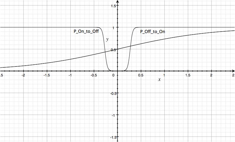
MSS Probabilities

Note that this plot looks very similar to the window function you will see in descriptions of other memristor models.

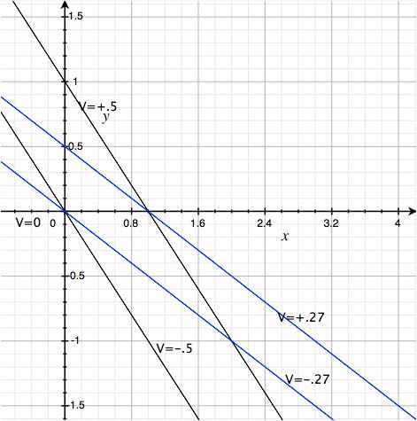
DX/dt as a Function of X at Different Applied Voltages

Here we plot the $dX/dt$ equation as a function of x at different applied voltages. The following plot shows a the correct behavior desired from the model:

If V=0, no change in X occurs
If V=+0.5V and X = 1, there will no more change (it’s already max.)
If V=+0.5V and X = 0, X will go to 1
If V=-0.5V and X = 1, X will go to 0 (dX=-1)
If V=-0.5V and X = 0, there will no more change (it’s already min.)

The same behavior occurs at the threshold voltages as well except that instead of at +/-1 change it’s at +/-0.5

MSS dX V0

One nice side effect of this model is that there are no extra checks on the bounds of X necessary like some other models. This is due to the Logistics function being bounded between 0 and 1.

Current as a Function of X

The final step to complete the MMSS model description is to define the current as a function of X. We can break that definition down into two steps, first the conductance, followed by the current. The conductance as a function of X is

$G = \frac{X}{ R_{ON} }+ \frac{1 - X}{R_{OFF}}$

Note that this describes a summation of conductances. Relating this to the real-world it tells us that our model is in fact 2 parallel resistors whose resistance values are coupled to each other via X.

For completeness, given a memristance value, for example $R_{init}$ ,

$X = \frac{R_{ON} (R_{init} - R_{OFF} )}{ R_{init} (R_{ON} - R_{OFF})}$

Finally, by Ohm’s Law the current is

$I = V \cdot G$

Preliminary Results in JSPICE

We call this new version of the MSS model the MMSS model, which stands for Mean Metastable Switch. Si\mulations comparing the original MSS and the new MMSS model in our own custom circuit si\mulator written is Java look the same, which is to be expected for large values of switches.

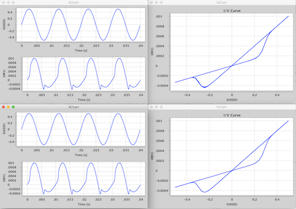
MSS vs MMSS Memristor Model

Given the results in JSPICE, I was confident that we could get this to work in Xyce.

Xyce Implementation

Most of the changes that were necessary for implementing this device in Xyce are exactly the same as in the previous post: Native Memristor Device Development in Xyce. The interesting portions of this device implementation are in the function Master::updateState and in the Sacdo templates.

Master::updateState

In this method I setup the two method calls to both I_V and dXdt

bool Master::updateState(double * solVec, double * staVec, double * stoVec)
{


  for (InstanceVector::const_iterator it = getInstanceBegin(); it != getInstanceEnd(); ++it)
  {
    Instance & ri = *(*it);
    
    double v_pos    = solVec[ri.li_Pos];
    double v_neg    = solVec[ri.li_Neg];
    double x        = solVec[ri.li_x];
        if (DEBUG_DEVICE){
            Xyce::dout()  << "  x_before = " <<  x << std::endl;
        }


        {
            Sacado::Fad::SFad<double,3> varV1( 3, 0, v_pos );
            Sacado::Fad::SFad<double,3> varV2( 3, 1, v_neg );
            Sacado::Fad::SFad<double,3> varX( 3, 2, x );
            Sacado::Fad::SFad<double,3> resultFad;
            resultFad = I_V( varV1, varV2, varX, ri.model_.Ron_, ri.model_.Roff_);

            ri.i0 = resultFad.val(); // current
            ri.G  = resultFad.dx(0); // di/dv = conductance
            ri.dIdx = resultFad.dx(2); // di/dx

        }

        {
            // evaluate the state variable equation
            Sacado::Fad::SFad<double,3> varV1( 3, 0, v_pos );
            Sacado::Fad::SFad<double,3> varV2( 3, 1, v_neg );
            Sacado::Fad::SFad<double,3> varX( 3, 2, x );
            Sacado::Fad::SFad<double,3> resultFad;

            // TODO make thermal voltage dynamic
            double vT = 0.026;
            resultFad = dXdt( varV1, varV2, varX, ri.model_.Ron_, ri.model_.Roff_, ri.model_.Von_, ri.model_.Voff_, ri.model_.\tau_, vT );

            ri.xVarFContribution = resultFad.val();
            if( getSolverState().dcopFlag )
            {
                ri.xVarFContribution = 0;
            }
            ri.dxFEqdVpos = resultFad.dx(0);
            ri.dxFEqdVneg = resultFad.dx(1);
            ri.dxFEqdx = resultFad.dx(2);

        }

  }

  return true;
}

bool Master::updateState(double * solVec, double * staVec, double * stoVec)

{

for (InstanceVector::const_iterator it = getInstanceBegin(); it != getInstanceEnd(); ++it)

{

Instance & ri = *(*it);

double v_pos = solVec[ri.li_Pos];

double v_neg = solVec[ri.li_Neg];

double x = solVec[ri.li_x];

if (DEBUG_DEVICE){

Xyce::dout() << " x_before = " << x << std::endl;

}

{

Sacado::Fad::SFad<double,3> varV1( 3, 0, v_pos );

Sacado::Fad::SFad<double,3> varV2( 3, 1, v_neg );

Sacado::Fad::SFad<double,3> varX( 3, 2, x );

Sacado::Fad::SFad<double,3> resultFad;

resultFad = I_V( varV1, varV2, varX, ri.model_.Ron_, ri.model_.Roff_);

ri.i0 = resultFad.val(); // current

ri.G = resultFad.dx(0); // di/dv = conductance

ri.dIdx = resultFad.dx(2); // di/dx

}

{

// evaluate the state variable equation

Sacado::Fad::SFad<double,3> varV1( 3, 0, v_pos );

Sacado::Fad::SFad<double,3> varV2( 3, 1, v_neg );

Sacado::Fad::SFad<double,3> varX( 3, 2, x );

Sacado::Fad::SFad<double,3> resultFad;

// TODO make thermal voltage dynamic

double vT = 0.026;

resultFad = dXdt( varV1, varV2, varX, ri.model_.Ron_, ri.model_.Roff_, ri.model_.Von_, ri.model_.Voff_, ri.model_.\tau_, vT );

ri.xVarFContribution = resultFad.val();

if( getSolverState().dcopFlag )

{

ri.xVarFContribution = 0;

}

ri.dxFEqdVpos = resultFad.dx(0);

ri.dxFEqdVneg = resultFad.dx(1);

ri.dxFEqdx = resultFad.dx(2);

}

return true;

}

Sacado Templates

Here are the Sacado templates used, which implement the bulk of the model.

template <typename ScalarT>
ScalarT p0ff2on( const ScalarT & V1, const ScalarT & V2, double VON, double TC, double VT )
{
    ScalarT exponent = -1 * ((V1-V2) - VON) / VT;
  double \alpha = 1 / TC;
  ScalarT fval = \alpha / (1.0 + exp(exponent));
  return fval;
}

template <typename ScalarT>
ScalarT pOn2Off( const ScalarT & V1, const ScalarT & V2, double VOFF, double TC, double VT )
{

    ScalarT exponent = -1 * ((V1-V2) + VOFF) / VT;
  double \alpha = 1 / TC;
  ScalarT fval = \alpha * (1.0 - 1.0 / (1.0 + exp(exponent)));
  return fval;
}

template <typename ScalarT>
ScalarT dXdt( const ScalarT & V1, const ScalarT & V2, const ScalarT & X, double RON, double ROFF, double VON, double VOFF, double TC, double VT)
{

  // Probabilities
    ScalarT p0ff2onVal = p0ff2on(V1, V2, VON, TC, VT);
    ScalarT pOn2OffVal = pOn2Off(V1, V2, VOFF, TC, VT);

  // Number of switches making a transition
    ScalarT n0ff2on = (1 - X) * p0ff2onVal;
    ScalarT nOn2Off = X  * pOn2OffVal;

    ScalarT fval = n0ff2on - nOn2Off;

    return fval;
}

template <typename ScalarT>

ScalarT p0ff2on( const ScalarT & V1, const ScalarT & V2, double VON, double TC, double VT )

{

ScalarT exponent = -1 * ((V1-V2) - VON) / VT;

double \alpha = 1 / TC;

ScalarT fval = \alpha / (1.0 + exp(exponent));

return fval;

}

template <typename ScalarT>

ScalarT pOn2Off( const ScalarT & V1, const ScalarT & V2, double VOFF, double TC, double VT )

{

ScalarT exponent = -1 * ((V1-V2) + VOFF) / VT;

double \alpha = 1 / TC;

ScalarT fval = \alpha * (1.0 - 1.0 / (1.0 + exp(exponent)));

return fval;

}

template <typename ScalarT>

ScalarT dXdt( const ScalarT & V1, const ScalarT & V2, const ScalarT & X, double RON, double ROFF, double VON, double VOFF, double TC, double VT)

{

// Probabilities

ScalarT p0ff2onVal = p0ff2on(V1, V2, VON, TC, VT);

ScalarT pOn2OffVal = pOn2Off(V1, V2, VOFF, TC, VT);

// Number of switches making a transition

ScalarT n0ff2on = (1 - X) * p0ff2onVal;

ScalarT nOn2Off = X * pOn2OffVal;

ScalarT fval = n0ff2on - nOn2Off;

return fval;

}

Xyce Si\mulation Results

The Xyce si\mulation file used to test the new MSS device follows.

* Voltage Sources
V1 1 0 SIN(0V 0.5V 100Hz)

* Memristors
YKNOWM mr1 1 0 mrm1 Rinit=500

.MODEL mrm1 knowm (level=1 Roff=1500 Ron=500 Voff=0.27 Von=0.27 \tau=0.0001)

* Analysis Command
.TRAN .1ms .04s
* Output
.PRINT TRAN V(1) I(V1) N(YKNOWM!mr1:R)

.END

* Voltage Sources

V1 1 0 SIN(0V 0.5V 100Hz)

* Memristors

YKNOWM mr1 1 0 mrm1 Rinit=500

.MODEL mrm1 knowm (level=1 Roff=1500 Ron=500 Voff=0.27 Von=0.27 \tau=0.0001)

* Analysis Command

.TRAN .1ms .04s

* Output

.PRINT TRAN V(1) I(V1) N(YKNOWM!mr1:R)

.END

Once rephrasing the MSS model in terms of $dX/dt$ , integration into Xyce was possible and pretty straight forward. The following screenshot shows the matching results from the above custom Java si\mulation.

MMSS Memristor Model in Xyce

Generalized Metastable Switch Model

In the Generalized model, the total current through the device comes from both a memory-dependent current component (MSS), $I_{m}$ , and a Schottky diode current, $I_{s}$ in parallel:

$I=\phi I_{m}(V,t)+(1-\phi)I_{s}(V)$

, where $\phi \in{[0,1]}$ . A value of $\phi=1$ represents a device that contains no Schottky diode effects.

We added the diode current component after realizing that the MSS component alone didn’t allow enough flexibility to fit a wide range of existing devices. After adding the diode component, we were able to fit data of a diverse range of memristors to the general model.

The Schottky component, $I_{s}(V)$ , follows from the fact that many memristive devices contain a Schottky barrier formed at a metal–semiconductor junction. The Schottky component is modeled by forward bias and reverse bias components as follows:

$I_{s}=\alpha_{f}e^{\beta_{f}V}-\alpha_{r}e^{-\beta_{r}V}$

, where $\alpha_{f}$ , $\beta_{f}$ , $\alpha_{r}$ , and $\beta_{r}$ are positive valued parameters setting the exponential behavior of the forward and reverse biases exponential current flow across the Schottky barrier.

Adding the Schottky component to our device model required minor effort including adding 5 new parameters, and modifying the I_V Sacado template as shown here:

template <typename ScalarT>
ScalarT SchottkyCurrent( const ScalarT & V1, const ScalarT & V2, double SchottkyForward\alpha, double SchottkyForward\beta, double SchottkyReverse\alpha, double SchottkyReverse\beta )
{
    return SchottkyReverse\alpha * (-1 * exp(-1 * SchottkyReverse\beta * (V1-V2))) + SchottkyForward\alpha * (exp(SchottkyForward\beta * (V1-V2)));
}

template <typename ScalarT>
ScalarT Geff( const ScalarT & X, double RON, double ROFF )
{
    return  X / RON + (1 - X) / ROFF;
}

template <typename ScalarT>
ScalarT I_V( const ScalarT & V1, const ScalarT & V2, const ScalarT & X, double RON, double ROFF, double PHI, double SchottkyForward\alpha, double SchottkyForward\beta, double SchottkyReverse\alpha, double SchottkyReverse\beta ){

    ScalarT Gval=   Geff( X, RON, ROFF );
    ScalarT MSSCurrentval = (V1-V2)*Gval;

    ScalarT SchottkyCurrentval = SchottkyCurrent(V1, V2, SchottkyForward\alpha, SchottkyForward\beta, SchottkyReverse\alpha, SchottkyReverse\beta);

    ScalarT fval = PHI * MSSCurrentval + (1 - PHI) * SchottkyCurrentval;

    return fval;
}

template <typename ScalarT>

ScalarT SchottkyCurrent( const ScalarT & V1, const ScalarT & V2, double SchottkyForward\alpha, double SchottkyForward\beta, double SchottkyReverse\alpha, double SchottkyReverse\beta )

{

return SchottkyReverse\alpha * (-1 * exp(-1 * SchottkyReverse\beta * (V1-V2))) + SchottkyForward\alpha * (exp(SchottkyForward\beta * (V1-V2)));

}

template <typename ScalarT>

ScalarT Geff( const ScalarT & X, double RON, double ROFF )

{

return X / RON + (1 - X) / ROFF;

}

template <typename ScalarT>

ScalarT I_V( const ScalarT & V1, const ScalarT & V2, const ScalarT & X, double RON, double ROFF, double PHI, double SchottkyForward\alpha, double SchottkyForward\beta, double SchottkyReverse\alpha, double SchottkyReverse\beta ){

ScalarT Gval= Geff( X, RON, ROFF );

ScalarT MSSCurrentval = (V1-V2)*Gval;

ScalarT SchottkyCurrentval = SchottkyCurrent(V1, V2, SchottkyForward\alpha, SchottkyForward\beta, SchottkyReverse\alpha, SchottkyReverse\beta);

ScalarT fval = PHI * MSSCurrentval + (1 - PHI) * SchottkyCurrentval;

return fval;

}

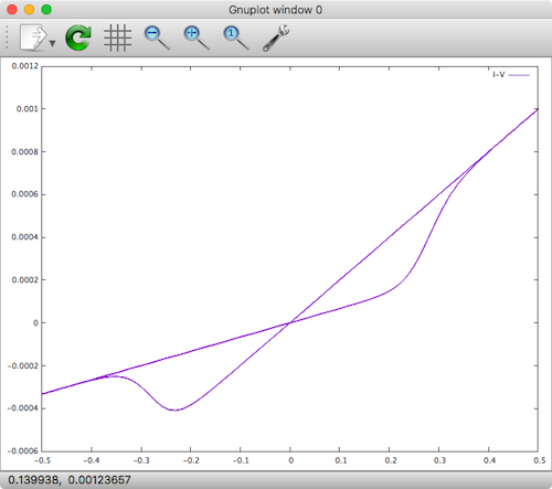
After recompiling and running the previous si\mulation with the modified model:

.MODEL mrm1 knowm (level=1 Roff=1500 Ron=500 Voff=0.27 Von=0.27 \tau=0.0001 PHI=0.8 SFA=0.0008 SFB=4 SRA=0.0008 SRB=4)

1 2	.MODEL mrm1 knowm (level=1 Roff=1500 Ron=500 Voff=0.27 Von=0.27 \tau=0.0001 PHI=0.8 SFA=0.0008 SFB=4 SRA=0.0008 SRB=4)

, the following hysteresis plot emerges.

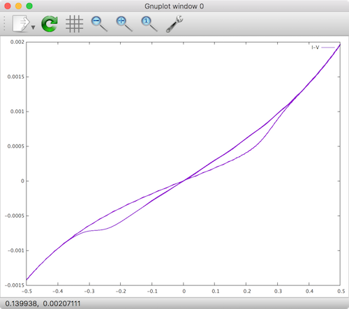
Generalized Metastable Switch Model

We can see that the addition of the forward and reverse Schottky diodes causes the shape of the forward and reverse current to take on a more exponential behavior. With this addition, fitting a very wide range of devices is possible, making it a good general model.

Conclusion

In this post I introduced the mathematics and implementation as a native device in Xyce of our generalized mean metastable switch (MMSS) memristor model. As a reminder, the model source files can be found at the memristor-models-4-all project on Github. Be sure to stay tuned by signing up for our newsletter and/or subscribing to our RSS feed to get the latest information about our memristor modeling progress. In the future, we will be blogging about more SPICE tools, other model implementations, and other memristor modeling advancements!

Memristor Modeling in Xyce

Model Conversion to dX/dt

Parameters

The Mean Metastable Switch Memristor Model

Visualization and Sanity Check

Probability as a Function of Voltage

DX/dt as a Function of X at Different Applied Voltages

Current as a Function of X

Preliminary Results in JSPICE

Xyce Implementation

Master::updateState

Sacado Templates

Xyce Si\mulation Results

Generalized Metastable Switch Model

Conclusion

Further Resources

Related Posts

Memristor Crossbars ...

Memristor Crossbars ...

How to embed XChart ...

Subscribe To Our Newsletter

Leave a Comment Cancel reply

Knowm Newsletter

Memristor Chips