This is an English translation to a two-part article that appeared in the German Physics Magazine “Physik in unserer Zeit” in early 2018. The original articles can be found at the following links: Jenseits des Mooreschen Gesetzes and Thermodynamisches Rechnen.
Abstract
While recent advances in the field of machine learning have begun to narrow the gap in algorithmic performance between nature’s brain and digital computers, a vast discrepancy remains in space, weight and power (SWaP). In order to significantly reduce this SWaP discrepancy, a radically new type of computer chip is necessary. Physics-based limitations arising from the separation of processor and memory in digital architecture, sometimes referred to as the von Neumann bottleneck, and the breakdown of Moore’s Law call for a new type of architecture where memory and processor unite and hardware becomes adaptive at the physical level. A type of computing called “Thermodynamic Computing”, distinct from classical and quantum, provides a theoretical foundation for a future where hardware becomes soft and SWaP performance equals and potentially surpasses biology.
Authors
Timothy W. Molter, M. Alexander Nugent
Introduction
Modern digital computers are arguably one of the most impressive inventions created by human beings and have enabled the proliferation of higher level technologies such as global telecommunication, the Internet and more recently machine learning and artificial intelligence, all of which have a profound influence on global economics and society as a whole. While the modern digital computer will continue to play an important and growing role in future technology, it contains a fundamental flaw in its design. When applied to large scale machine learning applications which require integrating and updating large numbers of synaptic weights or probabilities, it fails to scale [1]. For each integration of a synaptic weight in the network, the weight needs to be fetched from RAM, integrated in processor, and then placed back in RAM–over and over again. The limited data transfer rate between CPU and RAM, also known as the von Neumann bottleneck, and the associated energetic costs of communication grind a digital computing system to a halt as it attempts to scale up in size to match biology. While the energy expended in moving a bit in a modern integrated computer may be measured in nano or pico joules, a typical human cortex contains ~150,000,000,000,000 adaptive synapses. As digital computing systems ramp up data bandwidth and neural network sizes, the time and energy budgets quickly balloon beyond physical and financial constraints. While optimizations such as CPU core parallelization, faster and bigger CPU caches and transistor scaling can help, it is not enough. Incremental improvements over time, especially with the ending of Moore’s law in CMOS, are not going to span the gap between today’s digital computers and nature’s brain. The core problem is memory-processing separation, an invention of human ingenuity that is not found anywhere in nature. Just like GPUs act as a supplementary specialized processor for graphics, future machine learning processors will integrate into the existing technology stack and will accelerate machine learning by up to 9 orders of magnitude or more, reaching the efficiency found in biology.
Thermodynamics and the Temporal Evolution of Matter
If we completely forget everything we know about how modern computers work and attempted to design a new computer from scratch, we would probably first look at biology to see how it works, with the goal of reverse engineering it. This approach is what many cognitive neuroscience research efforts, such as the Human Brain Project, attempt to do. True North, Spinnaker, Deep Blue and Neurogrid are some examples of recent brain-inspired hardware that have resulted from such research efforts. Each architecture is fundamentally limited by the tools used to created it, namely the transistor, and the conceptual paradigm of memory-processor separation. All of these systems have failed to match primary (algorithmic) performance when compared to ML algorithms running on traditional digital processors as well as secondary (energy and space efficiency) performance when compared to biology. While the neuro-mimicry approach seems like a good approach at first, it is short sighted. Humans have a way of uncovering deeper principles in nature and using that understanding to create a new technology. The constraints of integrated electronics are radically different than the ionic action potentials in biological nervous systems. Just as we can learn from a bird about the concept of flight and apply this knowledge to the construction of a flying machine, so too can we learn from biology about the concept of physical adaptation and apply this knowledge to the construction of learning machines. The question becomes, what can we learn from nature about physical adaptation?
Thermodynamic computing was inspired from a fundamental property of nature – self organization and the laws of thermodynamics. In particular, it was inspired by a conundrum that many great minds have pondered. If the 2nd law says everything tends towards disorder, why does essentially everything we see in the universe contradict this? At almost every scale of the universe we see ordered self-organized structures, from black holes to stars, planets and suns to our own earth, the life that abounds on it and in particular the brain. Non-biological systems such as Benard convection cells, tornadoes, lightning and rivers, to name just a few, show us that matter does not tend toward disorder in practice but rather does quite the opposite. The standard answer is to point out that the 2nd law only applies to a closed system and the universe is not closed. While technically correct, it simply deepens the mystery: how does matter organize itself to produce the order we see in nature and in particular life?
Turing spent the last two years of his life working on mathematical biology and published a paper titled “The chemical basis of morphogenesis” in 1952 [2]. He was likely struggling with the concept that algorithms represent structure, brains and life in general are clearly capable of creating such structure, and brains are ultimately a biological chemical process that emerge from chemical homogeneity. How does complex spatial-temporal structure such as an algorithm emerge from the interaction of a homogeneous collection of units? In his 1944 lecture and book “What is Life?”, the father of Quantum Mechanics and Nobel laureate Erwin Schrödinger postulated that living matter evades the decay to thermodynamic equilibrium by maintaining ‘negative entropy’ in an open system [3]. That is, the reason a non-equilibrium structure does not dissolve is because it is dissipating free-energy and exporting entropy into the environment to counteract its own decay. In 1989 Swenson proposed and elaborated the Law of Maximum Entropy Production (LMEP) as the missing law that would account for the ubiquitous and opportunistic transformation from disordered, or less ordered, to more highly ordered states [4]. Along the same vein in 1996 Bejan began positioning his “Constructal Theory” as a new principle of thermodynamics and has since alluded to a “4th law of thermodynamics” [5]: “This ‘fourth law’ brings life and time explicitly into thermodynamics and creates a bridge between physics and biology.” In 2006, Morel et al. stated that “The Fourth Law leads to the expectation that dissipative structures will emerge in evolving systems [6]. Rather than being surprised, over and over again, when dissipative structures appear, chemists and biologists are advised to search for such spatially organized regions that facilitate entropy production.” Others including Sven Jorgensen, Jeremy England, Gavin Crooks, Alexander Wissner-Gross and Susanne Still are pushing forward the theory. Everybody appears to agree that ordered dissipative structures, including life, are allowed as long as they produce enough entropy to compensate for their own internal entropy reduction. Stated differently, ordered dissipative structures are entropy producing machines. For example, how would one build a container to hasten the spread of particles from a concentrated low-entropy state to a high-entropy state? A series of tubes in a binary fractal branching pattern such as machine “M” below is one such configuration. With this in mind we urge you to go out into nature and take a close look as to how it is built.
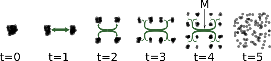
Machine M being used to speed up the transition of matter in a low-entropy configuration at t=0 to a high entropy configuration at t=5.
With practical uses of the 4th law on the horizon, it may soon become a first class citizen of the laws of thermodynamics. For us, the 4th law implies a profound conceptual insight and key constraint to building intrinsically adaptive computer chips because we think the answer to how brains organize themselves is ultimately the answer to how matter configures itself in nature. Indeed, it was a profound shock to us when we discovered that the same mechanisms postulated by the 4th law led directly to universal self-configuring logic, synaptic plasticity and foundational methods of machine learning.
Thermodynamic Bit (kT-bit)
Thermodynamic bits are points of energy-dissipating bifurcations. Trees, leaves, lighting, rivers, brains and circulatory systems are some examples of structure made of kT-bits, but there are many more. In fact, the only time you cannot see a thermodynamic bit is if you are inside a building or a city, away from nature and not looking in a mirror or at other living things. The non-obvious examples occur when you have two competing energy dissipating pathways but it does not look like a tree. The organs in you body, the organelles in cells and companies in our economy are some non-obvious examples. While they do not look like trees, they are competing adaptive energy dissipation flow structures nonetheless. In all cases there exists a particle that flows through the organization that is either a direct carrier of free-energy dissipation (electron, for example), or else gates-access to energy dissipation (blood, ATP, money, etc). In natural systems, the system (container of the flow) evolves automatically to adjust these competing flows in order to maximize energy dissipation. At each junction, two dissipation pathways compete for conduction resources. This building block is what we call a thermodynamic bit, and we have discovered that it is a universal adaptive computational building block.

Thermodynamic bits in nature allow living structures to dynamically adapt to maximize flow and in doing so increase the total entropy production in accordance with the second law of thermodynamics. We can create a synthetic thermodynamic bit with a pair of memristors.
To give a quick example of a thermodynamic bit evolving in time and space, take a tree branch with one single symmetric fork. Imagine that another tree grows in front of the branch, blocking the sunlight of all the leaves on one side of the fork. The side receiving more light will grow more relative to the side in the shade. The previously symmetric fork will now grow thicker in the direction leading to the sun, where the water taken up by the roots can evaporate into the sky. In this way, the tree adaptively grows into the optimal configuration to maximize flow (the 4th law) and in doing so increases entropy in accordance with the second law of thermodynamics.
Memristor
In electronics, we can create a thermodynamic bit with a pair of memristors. Memristors are “resistors with memory”. As a voltage is applied, the conductance will change. Just like any type of electronic component, there isn’t just one single memristor – there are many kinds made of different materials operating via different mechanisms, each having a unique set of properties. The most sought-after type of memristor is the bi-directional incremental variety. If you apply a positive voltage potential across the memristor with the lower potential on the end with the stripe, the memristor’s conductance will increase in proportion to the applied voltage and time, and it will decrease in conductance in an equivalent way for reverse voltage polarities. Applying a short positive voltage pulse will cause its conductance to increase slightly. Applying a short negative voltage pulse will cause its conductance to decrease slightly.
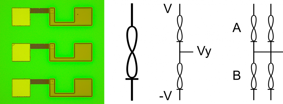
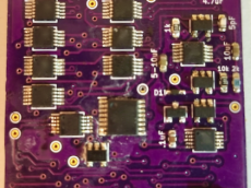
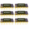
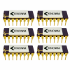
a) 3 Knowm memristors b) the memristor symbol c) a thermodynamic bit, also a voltage divider d) a thermodynamic neuron
Ohm’s Law, Voltage Divider
In addition to having a basic understanding of memristors, another key concept in understanding thermodynamic computing is Ohm’s Law: 
V is voltage, I is current and R is resistance. An alternative form, in terms of conductance is:

Most of the time, we refer to the conductance of a memristor rather than its resistance. Conductance is simply the inverse of resistance: 
A kT-bit can be made of two memristors connected in parallel or series, although below we will take a look at the series variety, which forms a simple voltage divider. When a voltage potential is applied across the two, some voltage less than the applied potential will be present at the node between the memristors:

When several kT-bits are connected to the same output node, 

y node (A) and bottom of the y node (B) respectively. Since the voltage, V, may be changed in a real circuit (for example to effect the adaptation rate), the (unit-less) value, y, can simply be normalized by the voltage:

Given the 3 electrodes (V, -V and Vy), there are several ways in which voltages could be applied to the kT-bit and we can list them all to create an instruction set. For sake of brevity, we will only list 4 instructions.
| Instruction | Applied Voltage Direction | Feedback | Applied Voltage to Vy node |
|---|---|---|---|
| FF | Forward | Float | None |
| RH | Reverse | High | -V |
| RL | Reverse | Low | +V |
| RU | Reverse | Unsupervised | -V if Vy > 0 else +V |
The applied voltage direction is the polarity of the voltage, V, across the synapse: current flows from the A-channel to the B-channel in the forward direction, and from the B-channel to the A-channel in the reverse direction.
The state of the kT-bit can be read with the FF instruction, and the voltage Vy is simply the result of the voltage division defined above. Note that as the kT-bit is being read the memristor conductances are adapting and the kT-bit’s output is incrementally driven towards zero. We call this an “Anti-Hebbian” instruction.
Feedback refers to how you wish to “teach” the kT-bit. If you want to teach the kT-bit to evaluate higher on the next read, then “high” feedback (RH) is applied and vice versa. “Unsupervised” feedback allows the kT-bit to decide for itself based on its prior read state. If it evaluates high during a FF operation, then an unsupervised operation (RU) will give feedback that reinforces its state. We call the RU instruction a “Hebbian” instruction.
An FF instruction followed by a RU instruction leads to Anti-Hebbian followed by Hebbian adaptation, or what we call the “unsupervised AHaH rule”.
Memristor conductance saturation occurs when it is pushed to its maximally-on or maximally-off state. In order to avoid saturation of both memristors in our kT-bit, a “flip-lock cycle” is utilized. During a read operation, if we apply a forward voltage (FF operation), the memristor conductance increases. To prevent saturation, this accumulation is compensated for via reverse polarity write voltages. Although there are exceptions, a good rule of thumb is to follow every forward-read operation by a reverse operation. In the table above we show a single forward read instruction and three reverse write instructions, but for every forward instruction there is a reverse instruction. For example, RF, FH, FL and FU.
Thermodynamic Neuron (kT-Neuron)
A thermodynamic neuron is formed when a collective of kT-bits are coupled to a common readout line, y. The functional objective of the kT-neuron is to produce an analog output signal on electrode y, given some arbitrary set of active kT-bits. Similar to a binary perceptron, an kT-neuron is able to linearly separate two classes of samples represented as n-dimensional input vectors. Unlike a perceptron, a kT-neuron is not an algorithm but an adaptive hardware construct, i.e. a physical adapting circuit where the output is an analog value representing the sum or integration of currents. Each kT-bit value (synaptic weight) is proportional to the difference in conductance between the memristors (
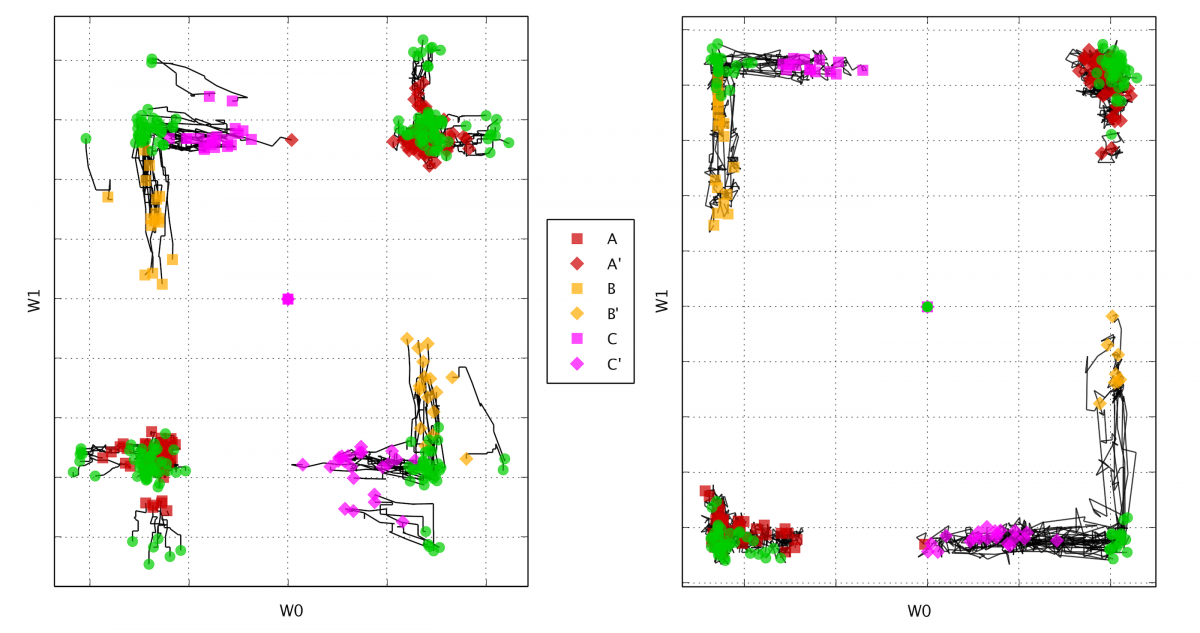
For real machine learning applications using kT-neurons, the typical number of kT-bits per neuron is in the hundreds to thousands. However with just two kT-bits we can demonstrate attractor dynamics leading to unsupervised learning and reconfigurable logic. Given a two-input kT-neuron, there are three possible ways to electrically couple the kT-bits to the y electrode [0,1], [1,0] or [1,1], where [1,1] indicates both kT-bits are coupled. If we randomly select patterns from the set, each with 1/3 probability and sequentially carry out FF and RU instruction for each pattern, we can observe the evolution of the kT-neuron over time.
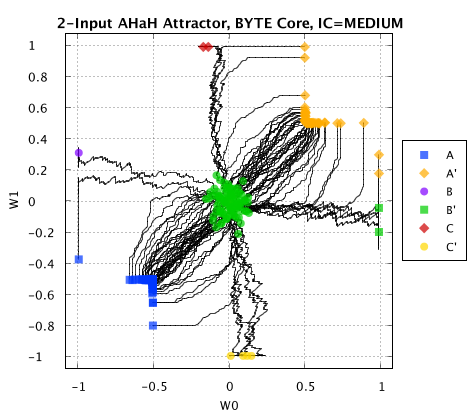
Unsupervised evolution of synaptic weights for a 2-input kT-neuron receiving 3 randomly selected input patterns [0,1], [1,0] or [1,1]. The final attractor basins determine how the neuron responds to new incoming data.
Analyzing the evolution of the synaptic weights for each trial, starting from the initial random distribution shown by the central green dots, we observe that the kT-neuron falls into 6 distinct attractor basins. The final state is driven by the initial random memristor conductances and the interaction of the kT-bits with each other as they adapt in accordance with the instructions. While in this simple experiment the synaptic states are driven by unsupervised evolution, in many machine learning applications the process is guided by external signals, i.e. supervised learning.
To understand these attractor states better, we can visualize the decision boundaries of this 2-input kT-neuron by solving the linear neuron equation for where the output, y, is zero:

This is the equation of a line, where the slope is given by the ratio of the two weights. Given a neuron with two synapses, we can plot it as a line on a 2D plane. Three synapses is a plane in 3D space and more than 3 synapses is a “hyperplane”. Every data point on one side of the hyperplane causes the neuron to output positive, and everything on the other side is negative. This hyperplane is called a decision boundary.
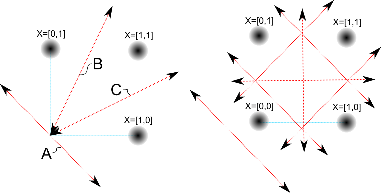
a) decision boundaries for a 2-input kT-neuron and three input patterns. b) decision boundaries for a 2-input kT-neuron and four input patterns.
Given two inputs that are spiking we have 3 possible patterns. Those are the black dots. The red lines are the decision boundaries of six different neurons that fell into 6 different attractor states, each representing a synaptic weight state and its anti-state, resulting in: A, !A, B, !B, C, !C, for a total of six states. Given a state (the arrow) and the right-hand rule, we can now just look at the diagram and see how the neuron will react–positive or negative–to each input spike pattern.
Truth table for 2-input 3-pattern decision boundaries
| State | [1,0] | [0,1] | [1,1] |
|---|---|---|---|
| A | – | – | – |
| !A | + | + | + |
| B | – | + | – |
| !B | + | – | + |
| C | – | + | + |
| !C | + | – | – |
Logic
Logic is the backbone of digital computing. If you take some number of discrete inputs and some number of discrete outputs, then it is possible to just list out all of the possible ways you can convert those inputs into outputs. That list is called “logic”, and each possible way is a ‘logic function’. For binary states there are 
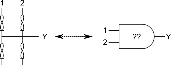
2-input kT-neuron as a 2-Input Self-Configuring Logic Gate
The 3 pattern attractor demonstration above can be extended to four or more patterns, and the attractor states cataloged to show that they are each distinct logic functions. In the case of this demonstration, the attractor state evolution was influenced by the random initialization, but in practice it can be influenced by a number of supervised and semi-supervised methods. Owing to the nature of fixed-point attractors, once the kT-neuron falls into a logic state, it stays there. Provide that information is processed, perturbations are repaired, a process akin to exercise and healing.
AHaH Rule
A synaptic plasticity rule defines how the synaptic weights in a neuron are updated when used and the AHaH (Anti-Hebbian and Hebbian) rule emerges from the flip-lock cycle, as we demonstrated above with the FF-RU instruction pair. The change to the synapse can be given as:
-\beta y")
, where 

")
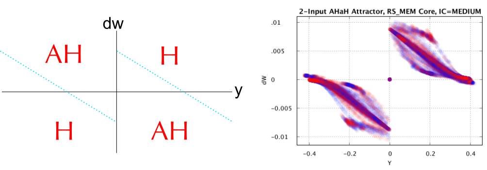
The AHaH (Anti-Hebbian and Hebbian) rule defines how each synaptic weight is updated depending on the neuron’s output value. Using different memristor types and instructions yield different physical rules, but they all tend to have the same general shape.
As y gets more positive, we transition from Hebbian (Quadrant 1) to Anti-Hebbian (Quadrant 2). Since we already know that Anti-Hebbian moves the weights toward zero, and Hebbian makes them grow, then it is not hard to see that we now have a stable rule: The weights grow quickly as first, then slow down and finally stop growing at some equilibrium value. It is exactly the same as y gets more negative. At first the weights get more negative quickly, but then they slow down until they hit an equilibrium value. The AHaH rule is like a wedge that attempts to bifurcate it’s data into two halves. However, it is the way in which this bifurcation occurs that you must understand. Low neuron activations (
AHaH Attractor States Obtained Experimentally with memristors
Putting It All Together
As we have just shown, we can create a thermodynamic bit out of two serially-connected memristors, which mimics a competing adaptive energy dissipation flow structure found throughout nature. Given an instruction set, which defines how voltages are applied to the kT-bit in the flip-lock cycle, we’ve demonstrated that a thermodynamic neuron formed of multiple kT-bits will fall into attractor basins that represent logic functions which maximize the margin between opposing data distributions. While we arrived at the dual memristor synapse from theoretical origins, practical considerations also lead one to converge on using kT-bits: Using two memristors rather than one allows for synaptic weights with both a state and magnitude. Additionally, using two memristors and the AHaH flip-lock cycle enables a convenient way to normalize all weights to zero despite memristor device variations arising from a non-ideal fabrication process. For other examples one can look at Joshua Yang’s recent dual-crossbar “competitive computing” architecture, Prezioso’s differential weight crossbars [7] and Truong’s dual-crossbar “winner take all” circuits [8]. For a more in-depth analysis of all aspects presented here as well as several machine learning demonstrations including unsupervised clustering, supervised and unsupervised classification, complex signal prediction, unsupervised robotic actuation and combinatorial optimization of procedures, see “AHaH Computing–From Metastable Switches to Attractors to Machine Learning” [9].
Summary
The brain functions fundamentally differently than a digital computer, and in order to build a computer which can achieve the space, weight and power performance as biology, a completely different approach needs to be taken where memory and processor are combined, eliminating the von Neumann bottleneck. Thermodynamic computing, relying on primitive thermodynamically-driven processes seen in energy dissipating structures throughout the universe, offers such a solution. We have presented our view of the fourth law of thermodynamics and its ability to explain the paradox between the second law of thermodynamics and the abundant contradictory ordered structure observed in nature. We believe that we are approaching a time where the fourth law will be gaining more attention and practical applications of it will be implemented, particularly in the field of computing and subsequently shedding light on Turing’s ideas of how algorithms can spontaneously form from homogeneous collections of units. By pairing memristors to create thermodynamic bits, chaining bits together to build thermodynamic neurons, connecting neurons into various topologies applicable to specific machine learning applications, and allowing them to evolve over time to maximize the flow of electrons, large scale physically self-organizing artificial intelligence systems are possible.
Keywords
Memristor, Rekonfigurierbares Logikgatter, Neuromorphics, Energieeffizienz, Lernfähiger Computer, Hauptsätze der Thermodynamik
References
[1] T. Potok et al., “Neuromorphic Computing Architectures, Models, and Applications.” 2016.
[2] A. Turing, “The chemical basis of morphogenesis.” Sciences-cecm. usp. br. 1952.
[3] E. Schrödinger, What is Life? Cambridge University Press, Cambridge 1944.
[4] R. Swenson, “Emergent attractors and the law of maximum entropy production: foundations to a theory of general evolution.” Systems Research and Behavioral Science 6.3 1989, 187-197.
[5] A. Bejan und G.W. Merkx, Constructal theory of social dynamics. New York: Springer 2007.
[6] R.E. Morel und G. Fleck. “A fourth law of thermodynamics.” Chemistry 15.4 2006, 305-310.
[7] M. Prezioso et al. “Training and operation of an integrated neuromorphic network based on metal-oxide memristors.” Nature 521.7550 2015, 61-64.
[8] S.N. Truong et al. “Ta2O5-memristor synaptic array with winner-take-all method for neuromorphic pattern matching.” Journal of the Korean Physical Society 69.4 2016, 640-646.
[9] M.A. Nugent und T.W. Molter “AHaH Computing–From Metastable Switches to Attractors to Machine Learning.” PloS one 9.2 2014, e85175.


2 Comments
Cere Davis
Hello.
Where can I find the English translation of this paper you published in PDF form?
https://doi.org/10.1002/piuz.201801485
Thanks.
Cere
Tim Molter
Sorry, but we don’t have it in PDF form. Just this web page!