Introduction

HelloTensorFlow aims to be a collection of notes, links, code snippets and mini-guides to teach you how to get Tensorflow up and running on MacOS (CPU only), Windows 10 (CPU and GPU) and Linux (work in progress) with zero experience in Tensorflow and little or no background in Python. It also runs through some basic machine learning code and concepts and focuses on specific details of TensorFlow as they are seen for the first time. This project assumes you are familiar with the command line, git and the most common developer tools of your chosen operating system. The code samples can be run in the console as is the most common scenario, but I also show how to set up Eclipse and the PyDev developer environment for Python motivated by my need for a cross platform IDE with code highlighting and other helpful IDE tools.

Many of the code examples have been taken from other Internet resources and credit is always given. We welcome pull requests for corrections, updates or additional tips, etc.

Before following along, take the time to read the Dev4Windows.md or Dev4MacOS.md to get things setup and installed and make sure you can successfully run hellopy.py and hellotf.py as well as some examples from the Tensorflow/models repo from the command line as well as from within Eclipse. The referenced dev instructions are also pasted in this blog post at the end of the walk through.

README

TF Walkthrough

The following 4 python (*.py) files are located in src and were adapted from Basic Concepts and Manipulations with TensorFlow. Reading the blog post, going through the code and comments and running the programs will familiarize you with the simplest Tensorflow concepts.

Linear Regression fits a line to a smattering of continuous X-Y values. At each iteration, the STG method is used along with the least squared error cost function. In this example the data is first normalized. linear_regression.py was adapted from Using Linear Regression in TensorFlow. Also see: Tensorflow API docs for Placeholders

linear_regression.py

Continuation

At this point we can leverage the project called TensorFlow-Examples to learn more M.L. in Tensorflow concepts. Go ahead and clone that repo and try running some of the examples either in the console or in Eclipse.

At this point, you could also use the Jupyter Notebook IDE for working with the examples, as it provides many nice conveniences although I’m quite happy with my Eclipse IDE setup.

python3 -m pip install jupyter
jupyter notebook

python3 -m pip install jupyter

jupyter notebook

Logistic Regression (logistic_regression.py)

Logistic Regression is like Linear Regression except it allows you to classify things rather than predict a continuous value. In logistic regression, the hypothesis function is the sigmoid function. The sigmoid function is bounded between 0 and 1, and produces a value that can be interpreted as a probability. This value can also be a yes / no answer with a cross-over, or decision boundary, at 0.5. The cost function is also changed from Linear Regression to be more compatible with gradient descent. The output is thresholded for a single class classifier and the softmax algo is used for a multi-class classifier.

A note on calculating model accuracy

Here is the “testing” code from the above example:

correct_prediction = tf.equal(tf.argmax(pred, 1), tf.argmax(y, 1))
# Calculate accuracy
accuracy = tf.reduce_mean(tf.cast(correct_prediction, tf.float32))
print("Accuracy:", accuracy.eval({x: mnist.test.images, y: mnist.test.labels}))

correct_prediction = tf.equal(tf.argmax(pred, 1), tf.argmax(y, 1))

# Calculate accuracy

accuracy = tf.reduce_mean(tf.cast(correct_prediction, tf.float32))

print("Accuracy:", accuracy.eval({x: mnist.test.images, y: mnist.test.labels}))

Argmax: Returns the index with the largest value across axes of a tensor.
axis (the 1 argument for the argmax function): A Tensor. Must be one of the following types: int32, int64. int32 or int64, must be in the range [-rank(input), rank(input)). Describes which axis of the input Tensor to reduce across. For vectors, use axis = 0.

In this case we have a matrix with rows representing the softmax score vector of the 10 digits for each test image. Axis = 0 refers to rows, axis = 1 refers to columns.

How do you use argmax and gather in Tensorflow?

correct_prediction = tf.equal(tf.argmax(pred, 1), tf.argmax(y, 1)): a matrix (10,000 rows by 1 column) of booleans representing the correct guess of the predictor according to the truth labels
accuracy = tf.reduce_mean(tf.cast(correct_prediction, tf.float32)): this converts the booleans to floats and calculates the mean of all elements in the matrix (tensor)

K-Means Clustering (kmeans.py)

For K-Means clustering, the concept is really simple. You pick K centroids and randomly place them. In a loop, you calculate the N closest datapoints to each centroid and calculate the average centroid location. Repeat until it converges. This converges to a local minimum so it is not at all perfect.

import os os.environ[“CUDA_VISIBLE_DEVICES”] = “”: Ignore all GPUs, tf random forest does not benefit from it. I think I read somewhere it’s even better to set it to -1. If you don’t set this and there is a GPU on the system it will run it on the GPU. This forces it to use the CPU.

Nearest Neighbor (nearest_neighbor.py)

In this example there is no training at all. You just give it a test image and all the “train” images and it sees which one it is closest to.

Random Forest (random_forest.py)

This demo uses the tensor_forest from the tf contrib package. It forms 10 trees, using the individual pixels as features. Each branch in the tree looks at the pixel values and makes a decision: left or right. The number of nodes in the trees is sqrt(numFeatures), and each node gathers statistics about the data it sees in order to determine an “optimal” threshold value for the decision. The outputs of all 10 trees are averaged to determine the combined classification output of the entire forest.

Again, here we ignore all GPUs, tf random forest does not benefit from it.

Saving and Importing a Model (save_restore_model.py)

Here the model is saved to disk and then restored later for inference use. It looks like the saving needs to be implemented in the Model itself.

model_path = "/tmp/model.ckpt"
# 'Saver' op to save and restore all the variables
saver = tf.train.Saver() // saves all variables, you could specify which ones.
...
# Save model weights to disk
save_path = saver.save(sess, model_path)
...
# Restore model weights from previously saved model
saver.restore(sess, model_path)

model_path = "/tmp/model.ckpt"

# 'Saver' op to save and restore all the variables

saver = tf.train.Saver() // saves all variables, you could specify which ones.

...

# Save model weights to disk

save_path = saver.save(sess, model_path)

...

# Restore model weights from previously saved model

saver.restore(sess, model_path)

When saving the model, you’ll notice there are 4 types of files:

“.meta” files: containing the graph structure
“.data” files: containing the values of variables
“.index” files: identifying the checkpoint
“checkpoint” file: a protocol buffer with a list of recent checkpoints

Checkpoints are binary files in a proprietary format which map variable names to tensor values. Savers can automatically number checkpoint filenames with a provided counter. This lets you keep multiple checkpoints at different steps while training a model.

A few other useful arguments of the Saver constructor, which enable control of the whole process, are:

max_to_keep: maximum number of checkpoints to keep,
keep_checkpoint_every_n_hours: a time interval for saving checkpoints

Tensorboard Basic (tensorboard_basic.py)

Tensorboard allows you to view the graph as well as model parameters, updating live.

logs_path = '/tmp/tensorflow_logs/example/'
...
# op to write logs to Tensorboard
summary_writer = tf.summary.FileWriter(logs_path, graph=tf.get_default_graph())
...
# Write logs at every iteration
summary_writer.add_summary(summary, epoch * total_batch + i)
...
print("Run the command line:\n" \
      "--> tensorboard --logdir=/tmp/tensorflow_logs " \
      "\nThen open http://0.0.0.0:6006/ into your web browser")

logs_path = '/tmp/tensorflow_logs/example/'

...

# op to write logs to Tensorboard

summary_writer = tf.summary.FileWriter(logs_path, graph=tf.get_default_graph())

...

# Write logs at every iteration

summary_writer.add_summary(summary, epoch * total_batch + i)

...

print("Run the command line:\n" \

"--> tensorboard --logdir=/tmp/tensorflow_logs " \

"\nThen open http://0.0.0.0:6006/ into your web browser")

Name scoping and nodes

Typical TensorFlow graphs can have many thousands of nodes–far too many to see easily all at once, or even to lay out using standard graph tools. To simplify, variable names can be scoped and the visualization uses this information to define a hierarchy on the nodes in the graph. By default, only the top of this hierarchy is shown. Here is an example that defines three operations under the hidden name scope using tf.name_scope:

import tensorflow as tf

with tf.name_scope('hidden') as scope:
  a = tf.constant(5, name='alpha')
  W = tf.Variable(tf.random_uniform([1, 2], -1.0, 1.0), name='weights')
  b = tf.Variable(tf.zeros([1]), name='biases')

import tensorflow as tf

with tf.name_scope('hidden') as scope:

a = tf.constant(5, name='alpha')

W = tf.Variable(tf.random_uniform([1, 2], -1.0, 1.0), name='weights')

b = tf.Variable(tf.zeros([1]), name='biases')

Grouping nodes by name scopes is critical to making a legible graph. If you’re building a model, name scopes give you control over the resulting visualization. The better your name scopes, the better your visualization.

Tensor shape information

When the serialized GraphDef includes tensor shapes, the graph visualizer labels edges with tensor dimensions, and edge thickness reflects total tensor size. To include tensor shapes in the GraphDef pass the actual graph object (as in sess.graph) to the FileWriter when serializing the graph.

Runtime statistics

Often it is useful to collect runtime metadata for a run, such as total memory usage, total compute time, and tensor shapes for nodes. The code example below is a snippet from the train and test section of a modification of the simple MNIST tutorial, in which we have recorded summaries and runtime statistics. See the Summaries Tutorial for details on how to record summaries. When you launch tensorboard and go to the Graph tab, you will now see options under “Session runs” which correspond to the steps where run metadata was added. Selecting one of these runs will show you the snapshot of the network at that step, fading out unused nodes. In the controls on the left hand side, you will be able to color the nodes by total memory or total compute time. Additionally, clicking on a node will display the exact total memory, compute time, and tensor output sizes.

  # Train the model, and also write summaries.
  # Every 10th step, measure test-set accuracy, and write test summaries
  # All other steps, run train_step on training data, & add training summaries

  def feed_dict(train):
    """Make a TensorFlow feed_dict: maps data onto Tensor placeholders."""
    if train or FLAGS.fake_data:
      xs, ys = mnist.train.next_batch(100, fake_data=FLAGS.fake_data)
      k = FLAGS.dropout
    else:
      xs, ys = mnist.test.images, mnist.test.labels
      k = 1.0
    return {x: xs, y_: ys, keep_prob: k}

  for i in range(FLAGS.max_steps):
    if i % 10 == 0:  # Record summaries and test-set accuracy
      summary, acc = sess.run([merged, accuracy], feed_dict=feed_dict(False))
      test_writer.add_summary(summary, i)
      print('Accuracy at step %s: %s' % (i, acc))
    else:  # Record train set summaries, and train
      if i % 100 == 99:  # Record execution stats
        run_options = tf.RunOptions(trace_level=tf.RunOptions.FULL_TRACE)
        run_metadata = tf.RunMetadata()
        summary, _ = sess.run([merged, train_step],
                              feed_dict=feed_dict(True),
                              options=run_options,
                              run_metadata=run_metadata)
        train_writer.add_run_metadata(run_metadata, 'step%d' % i)
        train_writer.add_summary(summary, i)
        print('Adding run metadata for', i)
      else:  # Record a summary
        summary, _ = sess.run([merged, train_step], feed_dict=feed_dict(True))
        train_writer.add_summary(summary, i)

# Train the model, and also write summaries.

# Every 10th step, measure test-set accuracy, and write test summaries

# All other steps, run train_step on training data, & add training summaries

def feed_dict(train):

"""Make a TensorFlow feed_dict: maps data onto Tensor placeholders."""

if train or FLAGS.fake_data:

xs, ys = mnist.train.next_batch(100, fake_data=FLAGS.fake_data)

k = FLAGS.dropout

else:

xs, ys = mnist.test.images, mnist.test.labels

k = 1.0

return {x: xs, y_: ys, keep_prob: k}

for i in range(FLAGS.max_steps):

if i % 10 == 0: # Record summaries and test-set accuracy

summary, acc = sess.run([merged, accuracy], feed_dict=feed_dict(False))

test_writer.add_summary(summary, i)

print('Accuracy at step %s: %s' % (i, acc))

else: # Record train set summaries, and train

if i % 100 == 99: # Record execution stats

run_options = tf.RunOptions(trace_level=tf.RunOptions.FULL_TRACE)

run_metadata = tf.RunMetadata()

summary, _ = sess.run([merged, train_step],

feed_dict=feed_dict(True),

options=run_options,

run_metadata=run_metadata)

train_writer.add_run_metadata(run_metadata, 'step%d' % i)

train_writer.add_summary(summary, i)

print('Adding run metadata for', i)

else: # Record a summary

summary, _ = sess.run([merged, train_step], feed_dict=feed_dict(True))

train_writer.add_summary(summary, i)

This code will emit runtime statistics for every 100th step starting at step 99.

Source and Code

A video to Watch

Hands-on TensorBoard (TensorFlow Dev Summit 2017)

We can do some amazing data mining, insight and comparison with TensorBoard. Also, we should be able to debug stuff like Nans Infs and Tensor shapes and data soon if not yet already.

Advanced Examples from TensorFlow-Examples

build_an_image_dataset.py – create a custom image dataset.
multigpu_basics.py – how to assign different parts of the graph to different GPUs.

Installation on MacOS

Main Tools

Create a directory called workspace_tf somewhere.
Install Sourcetree (optional)
Install Homebrew
Clone this repo (cd ~/path_to/workspace_tf, git clone https://github.com/Knowm/HelloTensorFlow.git)
brew cask install java
brew install python3
brew cask install eclipse-cpp or brew cask reinstall eclipse-cpp

PyDev in Eclipse

Create a workspace pointing to workspace_tf.
Install PyDev in Eclipse. Help ==> Install new Software… Click on Add… then PyDev in Name and http://pydev.org/updates/ in Location. Select PyDev and click through the wizard.
Configure PyDev in Eclipse preferences to point to installed Python executable. Go to Eclipse ==> Preferences ==> PyDev ==> Interpreter - Python Select New, set python3 and /usr/local/bin/python3

Import Python Project into Eclipse (PyDev)

Right click ==> New… ==> Project…
PyDev ==> PyDev Project ==> Next
Uncheck ‘Use Default’
Browse to project Directory
Copypasta Project Name
Next

Test Python in Eclipse

Right-click src/hellopy.py ==> Run As ==> Python Run

if __name__ == '__main__':
    print('Hello World')

if __name__ == '__main__':

print('Hello World')

Hello World

1 2	Hello World

Tensorflow

    pip3 install --upgrade tensorflow

1 2	pip3 install --upgrade tensorflow

Test TensorFlow in Eclipse

Right-click src/hellotf.py ==> Run As ==> Python Run

# https://mubaris.com/2017-10-21/tensorflow-101

# Import TensorFlow
import tensorflow as tf

# Define Constant
output = tf.constant("Hello, World")

# To print the value of constant you need to start a session.
sess = tf.Session()

# Print
print(sess.run(output))

# Close the session
sess.close()

# https://mubaris.com/2017-10-21/tensorflow-101

# Import TensorFlow

import tensorflow as tf

# Define Constant

output = tf.constant("Hello, World")

# To print the value of constant you need to start a session.

sess = tf.Session()

# Print

print(sess.run(output))

# Close the session

sess.close()

2017-11-17 10:33:55.587159: W tensorflow/core/platform/cpu_feature_guard.cc:45] The TensorFlow library wasn't compiled to use SSE4.2 instructions, but these are available on your machine and could speed up CPU computations.
2017-11-17 10:33:55.587179: W tensorflow/core/platform/cpu_feature_guard.cc:45] The TensorFlow library wasn't compiled to use AVX instructions, but these are available on your machine and could speed up CPU computations.
2017-11-17 10:33:55.587188: W tensorflow/core/platform/cpu_feature_guard.cc:45] The TensorFlow library wasn't compiled to use AVX2 instructions, but these are available on your machine and could speed up CPU computations.
2017-11-17 10:33:55.587192: W tensorflow/core/platform/cpu_feature_guard.cc:45] The TensorFlow library wasn't compiled to use FMA instructions, but these are available on your machine and could speed up CPU computations.
b'Hello, World'

2017-11-17 10:33:55.587159: W tensorflow/core/platform/cpu_feature_guard.cc:45] The TensorFlow library wasn't compiled to use SSE4.2 instructions, but these are available on your machine and could speed up CPU computations.

2017-11-17 10:33:55.587179: W tensorflow/core/platform/cpu_feature_guard.cc:45] The TensorFlow library wasn't compiled to use AVX instructions, but these are available on your machine and could speed up CPU computations.

2017-11-17 10:33:55.587188: W tensorflow/core/platform/cpu_feature_guard.cc:45] The TensorFlow library wasn't compiled to use AVX2 instructions, but these are available on your machine and could speed up CPU computations.

2017-11-17 10:33:55.587192: W tensorflow/core/platform/cpu_feature_guard.cc:45] The TensorFlow library wasn't compiled to use FMA instructions, but these are available on your machine and could speed up CPU computations.

b'Hello, World'

MNIST from `Tensorflow/models`

cd ~/path_to/workspace_tf
git clone https://github.com/tensorflow/models.git
python3 models/tutorials/image/mnist/convolutional.py

cd ~/path_to/workspace_tf

git clone https://github.com/tensorflow/models.git

python3 models/tutorials/image/mnist/convolutional.py

Alternatively, import the models project into Eclipse as described above for HelloTensorFlow, right-click tutorials/image/mnist/convolutional.py ==> Run As ==> Python Run.

Cifar-10 from `Tensorflow/models`

cd ~/path_to/workspace_tf
python3 models/tutorials/image/cifar10/cifar10_train.py

cd ~/path_to/workspace_tf

python3 models/tutorials/image/cifar10/cifar10_train.py

In a different console window:

tensorboard --logdir=/tmp/cifar10_train

1 2	tensorboard --logdir=/tmp/cifar10_train

Open http://localhost:6006 in browser to view tensorboard.

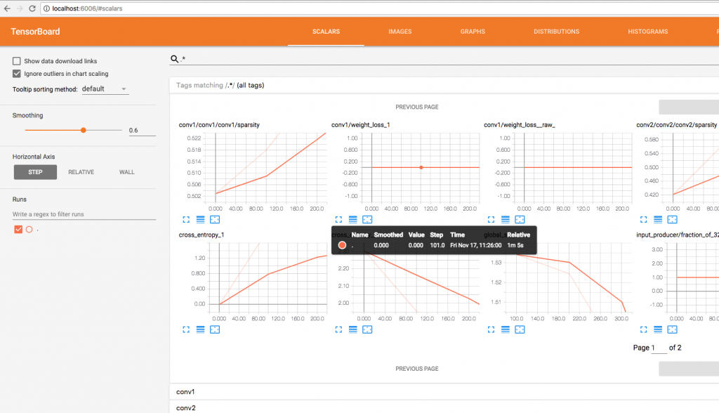
Tensorflow MacOSTensorboard

After training and monitoring on tensorboard:

python3 cifar10_eval.py

1 2	python3 cifar10_eval.py

Results on Mac (CPU only)

Device	Info
CPU	Intel i5 2.9 GHz
RAM	Apple 8GB DDR3 1867 MHz 2 core

Running 5000 steps on the CPU took 57 minutes.

Installation on Windows 10

Main Tools

Create a directory called workspace_tf somewhere.
Install Sourcetree
Clone this repo (cd ~/path_to/workspace_tf, git clone https://github.com/Knowm/HelloTensorFlow.git)
Install Git-Gui (for command line stuff)
Install Java8
Install Python
Install Eclipse

Python

Create a workspace pointing to workspace_tf.
Install PyDev in Eclipse. Help ==> Install new Software… Click on Add… then PyDev in Name and http://pydev.org/updates/ in Location. Select PyDev and click through the wizard.
Configure PyDev in Eclipse preferences to point to installed Python executable. Go to Window ==> Preferences ==> PyDev ==> Interpreter - Python Select Qucik auto-Config and it should find python automatically.

Import Python Project into Eclipse (PyDev)

Right click ==> New… ==> Project…
PyDev ==> PyDev Project ==> Next
Uncheck ‘Use Default’
Browse to project Directory
Copypasta Project Name
Next

To get Python to run from the command line, open up the command promt (type cmd), then:

c:/Path/to/AppData/Local/Programs/Python/Python36/Tools/scripts/win_add2path.py

1 2	c:/Path/to/AppData/Local/Programs/Python/Python36/Tools/scripts/win_add2path.py

This adds all the correct paths to the $PATH.

Test Python in Eclipse

Right-click hellopy.py ==> Run As ==> Python Run

if __name__ == '__main__':
    print('Hello World')

if __name__ == '__main__':

print('Hello World')

Hello World

1 2	Hello World

CUDA and CUDNN

CUDA installation guide
Nvidia recommends installing Visual Studio so why not? Will come in handy later if developing GPU code.

The official Tensorflow 1.4 builds require CUDA 8 and CuDNN 6, so don’t install the latest and greatest.

Download and install Cuda 8 Toolkit (Do the base install and the patch afterwards)
Download CuDNN 6 Toolkit (requires nvidia developer account)
Follow install [instructions] 1-3 (http://docs.nvidia.com/deeplearning/sdk/cudnn-install/index.html) (adapt for CUDA 8 and CuDNN 6) Follow additional instructions later for CuDNN dev, but not needed for TF.

TensorFlow

Open up the command promt (type cmd)
python -m pip install --upgrade pip
pip install --upgrade tensorflow-gpu

Test TensorFlow in Eclipse

Right-click hellotf.py ==> Run As ==> Python Run

# https://mubaris.com/2017-10-21/tensorflow-101

# Import TensorFlow
import tensorflow as tf

# Define Constant
output = tf.constant("Hello, World")

# To print the value of constant you need to start a session.
sess = tf.Session()

# Print
print(sess.run(output))

# Close the session
sess.close()

# https://mubaris.com/2017-10-21/tensorflow-101

# Import TensorFlow

import tensorflow as tf

# Define Constant

output = tf.constant("Hello, World")

# To print the value of constant you need to start a session.

sess = tf.Session()

# Print

print(sess.run(output))

# Close the session

sess.close()

2017-11-17 08:56:23.787312: I C:\tf_jenkins\home\workspace\rel-win\M\windows-gpu\PY\36\tensorflow\core\platform\cpu_feature_guard.cc:137] Your CPU supports instructions that this TensorFlow binary was not compiled to use: AVX AVX2
2017-11-17 08:56:23.982426: I C:\tf_jenkins\home\workspace\rel-win\M\windows-gpu\PY\36\tensorflow\core\common_runtime\gpu\gpu_device.cc:1030] Found device 0 with properties: 
name: GeForce GTX 1080 major: 6 minor: 1 memoryClockRate(GHz): 1.8225
pciBusID: 0000:01:00.0
totalMemory: 8.00GiB freeMemory: 6.66GiB
2017-11-17 08:56:23.982655: I C:\tf_jenkins\home\workspace\rel-win\M\windows-gpu\PY\36\tensorflow\core\common_runtime\gpu\gpu_device.cc:1120] Creating TensorFlow device (/device:GPU:0) -&gt; (device: 0, name: GeForce GTX 1080, pci bus id: 0000:01:00.0, compute capability: 6.1)
b'Hello, World'

2017-11-17 08:56:23.787312: I C:\tf_jenkins\home\workspace\rel-win\M\windows-gpu\PY\36\tensorflow\core\platform\cpu_feature_guard.cc:137] Your CPU supports instructions that this TensorFlow binary was not compiled to use: AVX AVX2

2017-11-17 08:56:23.982426: I C:\tf_jenkins\home\workspace\rel-win\M\windows-gpu\PY\36\tensorflow\core\common_runtime\gpu\gpu_device.cc:1030] Found device 0 with properties:

name: GeForce GTX 1080 major: 6 minor: 1 memoryClockRate(GHz): 1.8225

pciBusID: 0000:01:00.0

totalMemory: 8.00GiB freeMemory: 6.66GiB

2017-11-17 08:56:23.982655: I C:\tf_jenkins\home\workspace\rel-win\M\windows-gpu\PY\36\tensorflow\core\common_runtime\gpu\gpu_device.cc:1120] Creating TensorFlow device (/device:GPU:0) -> (device: 0, name: GeForce GTX 1080, pci bus id: 0000:01:00.0, compute capability: 6.1)

b'Hello, World'

MNIST from `Tensorflow/models`

Open up the Git command prompt (not cmd!)

cd ~/path_to/workspace_tf
git clone https://github.com/tensorflow/models.git
python models/tutorials/image/mnist/convolutional.py

cd ~/path_to/workspace_tf

git clone https://github.com/tensorflow/models.git

python models/tutorials/image/mnist/convolutional.py

Alternatively, import the models project into Eclipse as described above for HelloTensorFlow, right-click tutorials/image/mnist/convolutional.py ==> Run As ==> Python Run.

Force to run on CPU (disable GPU)

Open up models/tutorials/image/mnist/convolutional.py.
Add…

import os
os.environ["CUDA_VISIBLE_DEVICES"]="-1" # this disables the GPU and it will run on the CPU only, set to "0" for GPU
from tensorflow.python.client import device_lib
print(device_lib.list_local_devices())

import os

os.environ["CUDA_VISIBLE_DEVICES"]="-1" # this disables the GPU and it will run on the CPU only, set to "0" for GPU

from tensorflow.python.client import device_lib

print(device_lib.list_local_devices())

CPU vs GPU

Running on the CPU took 25 minutes, while running on the GPU took 14 minutes.

Cifar-10

Open up the Git command prompt (not cmd!)

cd ~/path_to/workspace_tf
python models/tutorials/image/cifar10/cifar10_train.py

cd ~/path_to/workspace_tf

python models/tutorials/image/cifar10/cifar10_train.py

In a different console window:

tensorboard --logdir=/tmp/cifar10_train

1 2	tensorboard --logdir=/tmp/cifar10_train

Open the link it gives you in browser to view tensorboard.

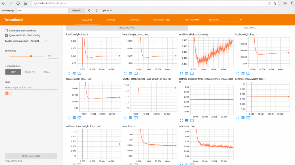
Tensorflow Windows 10 Tensorboard

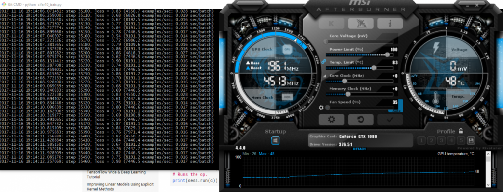
Tensorflow Windows 10 GPU

After training and monitoring on tensorboard:

python models/tutorials/image/cifar10/cifar10_eval.py

1 2	python models/tutorials/image/cifar10/cifar10_eval.py

Results on Windows CPU vs GPU

Device	Info
CPU	Intel i7-7700K 4.20 GHz 8 core
GPU	NVidia 1080 8GB
RAM	Apple 32GB DDR4 3200 MHz

Running 5000 steps on the CPU took 28 minutes, while running on the GPU took a little over a minute for a 19.7x performance increase!

Machine Learning with Tensorflow for Beginners – How to Install, Run and Understand Basic Machine Learning Demos

Introduction

README

TF Walkthrough

Continuation

Logistic Regression (logistic_regression.py)

A note on calculating model accuracy

K-Means Clustering (kmeans.py)

Nearest Neighbor (nearest_neighbor.py)

Random Forest (random_forest.py)

Saving and Importing a Model (save_restore_model.py)

Tensorboard Basic (tensorboard_basic.py)

Name scoping and nodes

Tensor shape information

Runtime statistics

A video to Watch

Advanced Examples from TensorFlow-Examples

Installation on MacOS

Main Tools

PyDev in Eclipse

Import Python Project into Eclipse (PyDev)

Test Python in Eclipse

Tensorflow

Test TensorFlow in Eclipse

MNIST from Tensorflow/models

Cifar-10 from Tensorflow/models

Results on Mac (CPU only)

Installation on Windows 10

Main Tools

Python

Import Python Project into Eclipse (PyDev)

Test Python in Eclipse

CUDA and CUDNN

TensorFlow

Test TensorFlow in Eclipse

MNIST from Tensorflow/models

Force to run on CPU (disable GPU)

CPU vs GPU

Cifar-10

Results on Windows CPU vs GPU

Memristor Crossbars ...

Memristor Crossbars ...

How to embed XChart ...

Leave a Comment Cancel reply

MNIST from `Tensorflow/models`

Cifar-10 from `Tensorflow/models`

MNIST from `Tensorflow/models`