AHaH Computing–From Metastable Switches to Attractors to Machine Learning

Abstract

Modern computing architecture based on the separation of memory and processing leads to a well known problem called the von Neumann bottleneck, a restrictive limit on the data bandwidth between CPU and RAM. This paper introduces a new approach to computing we call AHaH computing where memory and processing are combined. The idea is based on the attractor dynamics of volatile dissipative electronics inspired by biological systems, presenting an attractive alternative architecture that is able to adapt, self-repair, and learn from interactions with the environment. We envision that both von Neumann and AHaH computing architectures will operate together on the same machine, but that the AHaH computing processor may reduce the power consumption and processing time for certain adaptive learning tasks by orders of magnitude. The paper begins by drawing a connection between the properties of volatility, thermodynamics, and Anti-Hebbian and Hebbian (AHaH) plasticity. We show how AHaH synaptic plasticity leads to attractor states that extract the independent components of applied data streams and how they form a computationally complete set of logic functions. After introducing a general memristive device model based on collections of metastable switches, we show how adaptive synaptic weights can be formed from differential pairs of incremental memristors. We also disclose how arrays of synaptic weights can be used to build a neural node circuit operating AHaH plasticity. By configuring the attractor states of the AHaH node in different ways, high level machine learning functions are demonstrated. This includes unsupervised clustering, supervised and unsupervised classification, complex signal prediction, unsupervised robotic actuation and combinatorial optimization of procedures—all key capabilities of biological nervous systems and modern machine learning algorithms with real world application.

Introduction

How does nature compute? Attempting to answer this question naturally leads one to consider biological nervous systems, although examples of computation abound in other manifestations of life. Some examples include plants, bacteria, protozoan, and swarms, to name a few. Most attempts to understand biological nervous systems fall along a spectrum. One end of the spectrum attempts to mimic the observed physical properties of nervous systems. These models necessarily contain parameters that must be tuned to match the biophysical and architectural properties of the natural model. Examples of this approach include Boahen’s neuromorphic circuit at Stanford University and their Neurogrid processor, the mathematical spiking neuron model of Izhikevich as well as the large scale modeling of Eliasmith. The other end of the spectrum abandons biological mimicry in an attempt to algorithmically solve the problems associated with brains such as perception, planning and control. This is generally referred to as machine learning. Algorithmic examples include support vector maximization, k-means clustering and random forests. Many approaches fall somewhere along the spectrum between mimicry and machine learning, such as the CAVIAR and Cognimem neuromorphic processors as well as IBM’s neurosynaptic core. In this paper we consider an alternative approach outside of the typical spectrum by asking ourselves a simple but important question: How can a brain compute given that it is built of volatile components?

A brain, like all living systems, is a far-from-equilibrium energy dissipating structure that constantly builds and repairs itself. We can shift the standard question from “how do brains compute?” or “what is the algorithm of the brain?” to a more fundamental question of “how do brains build and repair themselves as dissipative attractor-based structures?”

Just as a ball will roll into a depression, an attractor-based system will fall into its attractor states. Perturbations (damage) will be fixed as the system reconverges to its attractor state. As an example, if we cut ourselves we heal. To bestow this property on our computing technology we must find a way to represent our computing structures as attractors. In this paper we detail how the attractor points of a plasticity rule we call Anti-Hebbian and Hebbian (AHaH) plasticity are computationally complete logic functions as well as building blocks for machine learning functions. We further show that AHaH plasticity can be attained from simple memristive circuitry attempting to maximize circuit power dissipation in accordance with ideas in nonequilibrium thermodynamics.

Our goal is to lay a foundation for a new type of practical computing based on the configuration and repair of volatile switching elements. We traverse the large gap from volatile memristive devices to demonstrations of computational universality and machine learning. The reader should keep in mind that the subject matter in this paper is necessarily diverse, but is essentially an elaboration of these three points:

1. AHaH plasticity emerges from the interaction of volatile competing energy dissipating pathways.
2. AHaH plasticity leads to attractor states that can be used for universal computation and advanced machine learning
3. Neural nodes operating AHaH plasticity can be constructed from simple memristive circuits.

…

Read the entire article one the web at http://dx.plos.org/10.1371/journal.pone.0085175.

Select Figures

AHaH Computing

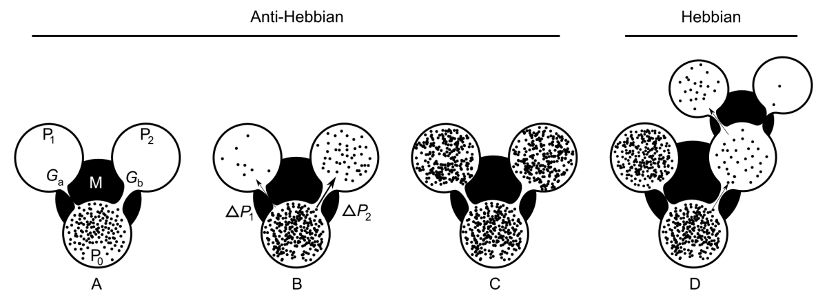
Fig. 1. AHaH process. A) A first replenished pressurized container P_0 is allowed to diffuse into two non-pressurized empty containers P_1 and P_2 though a region of matter M. B) The gradient dP_2 reduces faster than the gradient dP_1 due to the conductance differential. C) This causes G_a to grow more than G_b, reducing the conductance differential and leading to anti-Hebbian learning. D) The first detectable signal (work) is available at P_2 owing to the differential that favors it. As a response to this signal, events may transpire in the environment that open up new pathways to particle dissipation. The initial conductance differential is reinforced leading to Hebbian learning.

Attractor states of a two-input AHaH node

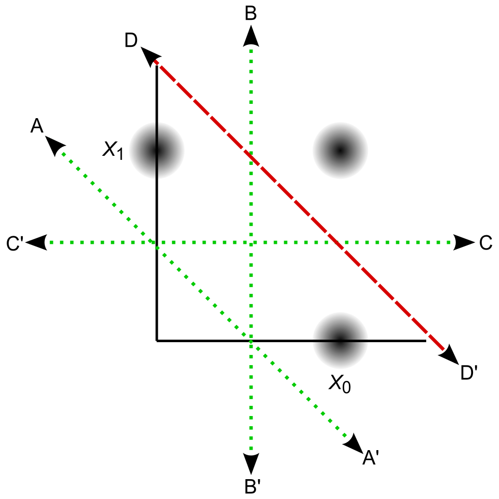
Fig. 2. Attractor states of a two-input AHaH node. The AHaH rule naturally forms decision boundaries that maximize the margin between data distributions (black blobs). This is easily visualized in two dimensions, but it is equally valid for any number of inputs. Attractor states are represented by decision boundaries A, B, C (green dotted lines) and D (red dashed line). Each state has a corresponding anti-state. State A is the null state and its occupation is inhibited by the bias. State D has not yet been reliably achieved in circuit simulations.

A differential pair of memristors forms a synapse.

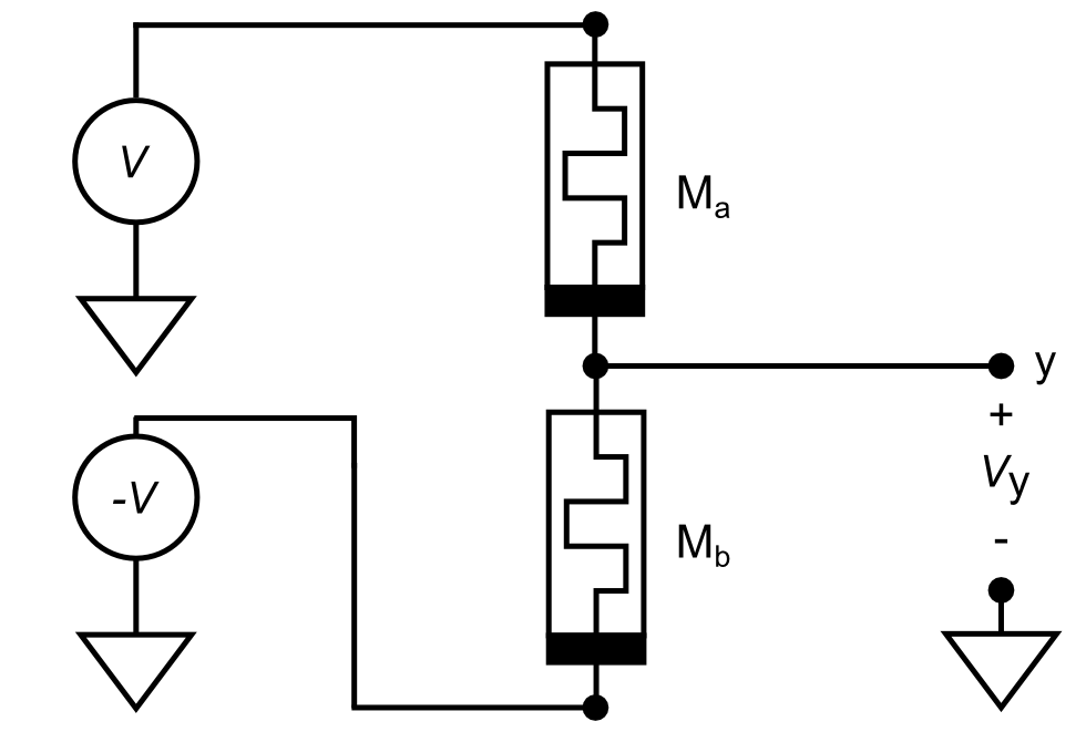
Fig. 4. A differential pair of memristors forms a synapse. A differential pair of memristors is used to form a synaptic weight, allowing for both a sign and magnitude. The bar on the memristor is used to indicate polarity and corresponds to the lower potential end when driving the memristor into a higher conductance state. M_a and M_b form a voltage divider causing the voltage at node y to be some value between V and -V. When driven correctly in the absence of Hebbian feedback a synapse will evolve to a symmetric state where V_y = 0 V, alleviating issues arising from device inhomogeneities.

AHaH 2-1 two-phase circuit diagram

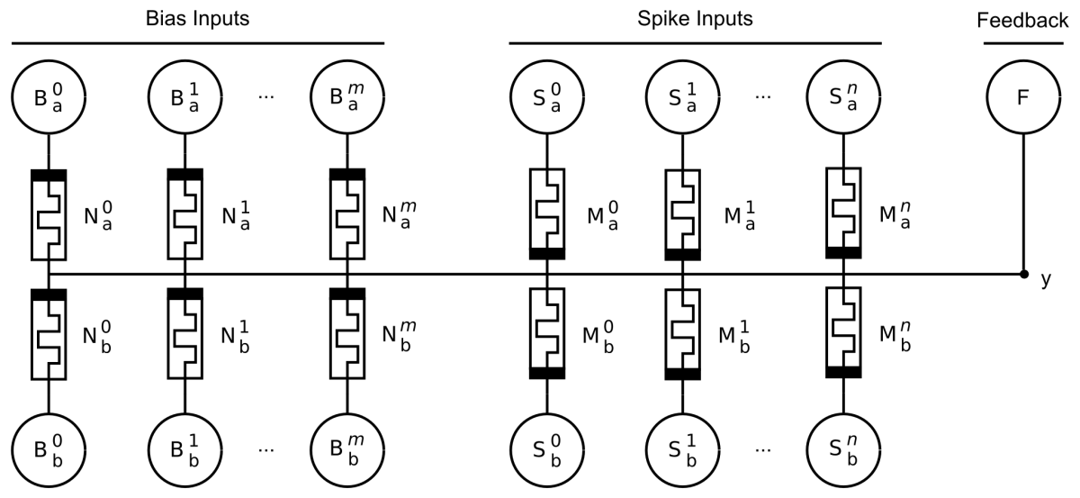
Fig. 5. AHaH 2-1 two-phase circuit diagram. The circuit produces an analog voltage signal on the output at node y given a spike pattern on its inputs labeled S^0, S^1 …, S^n. The bias inputs B^0, B^1 …, B^m are equivalent to the spike pattern inputs except that they are always active when the spike pattern inputs are active. F is a voltage source used to implement supervised and unsupervised learning via the AHaH rule. The polarity of the memristors for the bias synapse(s) is inverted relative to the input memristors. The output voltage, V_y, contains both state (positive/negative) and confidence (magnitude) information.

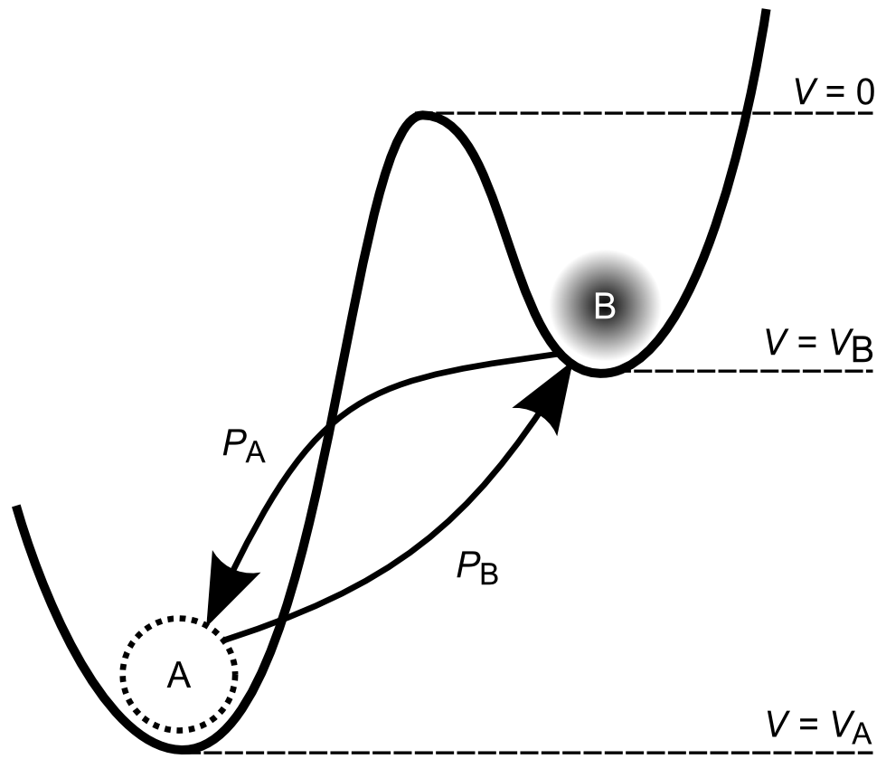
Generalized Metastable Switch (MSS) Memristor Model

Fig. 7. Generalized Metastable Switch (MSS). An MSS is an idealized two-state element that switches probabilistically between its two states as a function of applied voltage bias and temperature. The probability that the MSS will transition from the B state to the A state is given by P_A, while the probability that the MSS will transition from the A state to the B state is given by P_B. We model a memristor as a collection of $N$ MSSs evolving over discrete time steps.

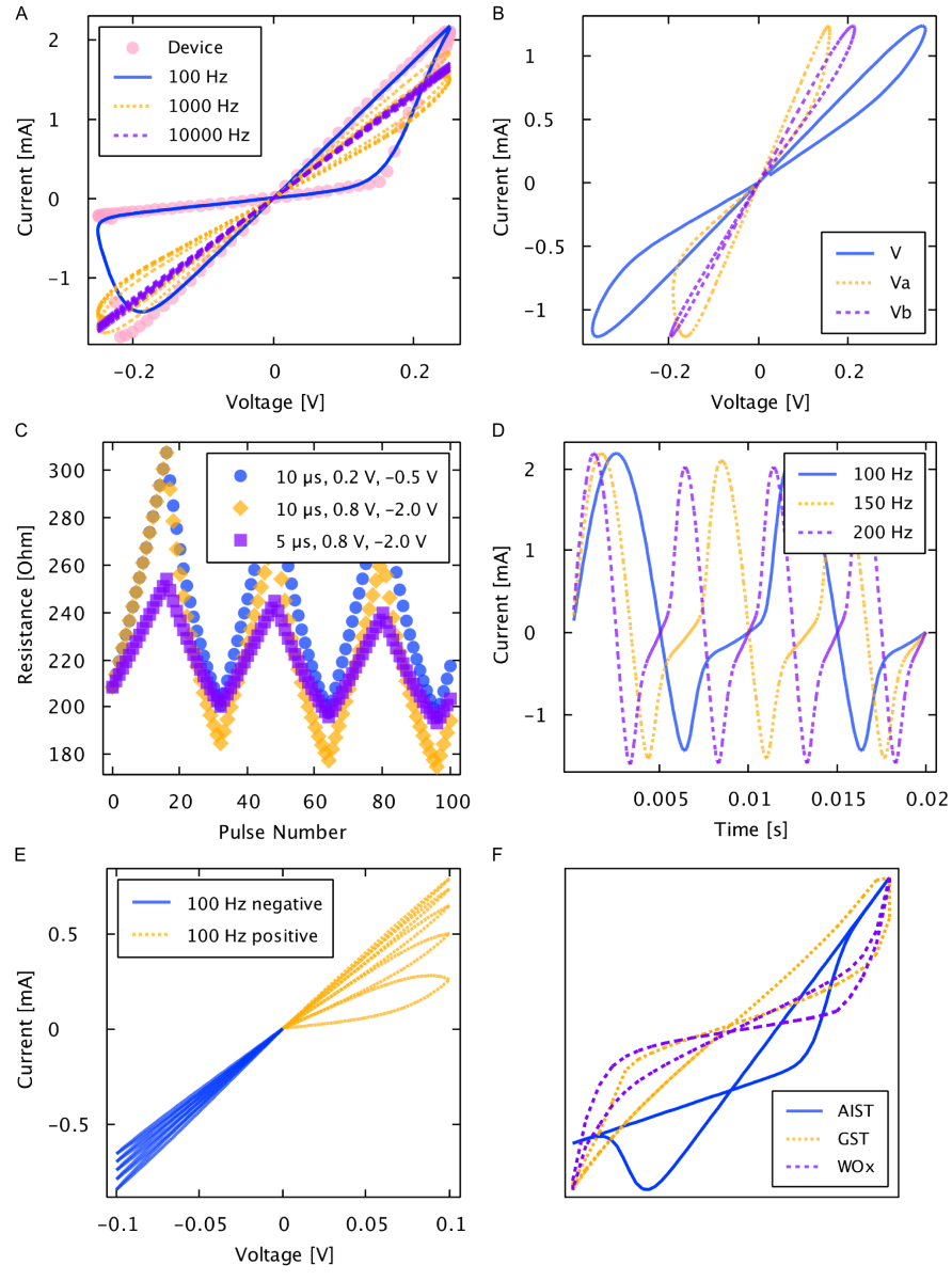
Generalized memristive device model simulations

Fig. 8. Generalized memristive device model simulations. A) Solid line represents the model simulated at 100~Hz and dots represent the measurements from a physical Ag-chalcogenide device from Boise State University. Physical and predicted device current resulted from driving a sinusoidal voltage of 0.25 V amplitude at 100 Hz across the device. B) Simulation of two series-connected arbitrary devices with differing model parameter values. C) Simulated response to pulse trains of 10 µs, 0.2 V, -0.5 V, 10 µs, 0.8 V, -2.0 V, and 5 µs, 0.8 V, -2.0 V showing the incremental change in resistance in response to small voltage pulses. D) Simulated time response of model from driving a sinusoidal voltage of 0.25 V amplitude at 100 Hz, 150 Hz, and 200 Hz. E) Simulated response to a triangle wave of 0.1 V amplitude at 100 Hz showing the expected incremental behavior of the model. F) Simulated and scaled hysteresis curves for the AIST, GST, and WO_x devices (not to scale).

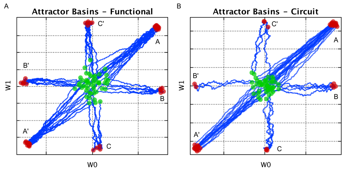
Attractor states of a two-input AHaH node

Fig. 12. Attractor states of a two-input AHaH node under the three-pattern input. The AHaH rule naturally forms decision boundaries that maximize the margin between data distributions. Weight space plots show the initial weight coordinate (green circle), the final weight coordinate (red circle) and the path between (blue line). Evolution of weights from a random normal initialization to attractor basins can be clearly seen for both the functional model (A) and circuit model (B).

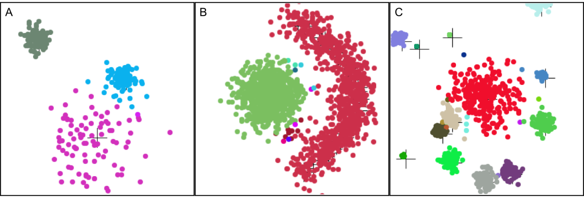
Two-dimensional spatial clustering demonstrations

Fig. 15 Two-dimensional spatial clustering demonstrations. The AHaH clusterer performs well across a wide range of different 2D spatial cluster types, all without predefining the number of clusters or the expected cluster types. A) Gaussian B) non-Gaussian C) random Gaussian size and placement.

AHaH Classification benchmarks results

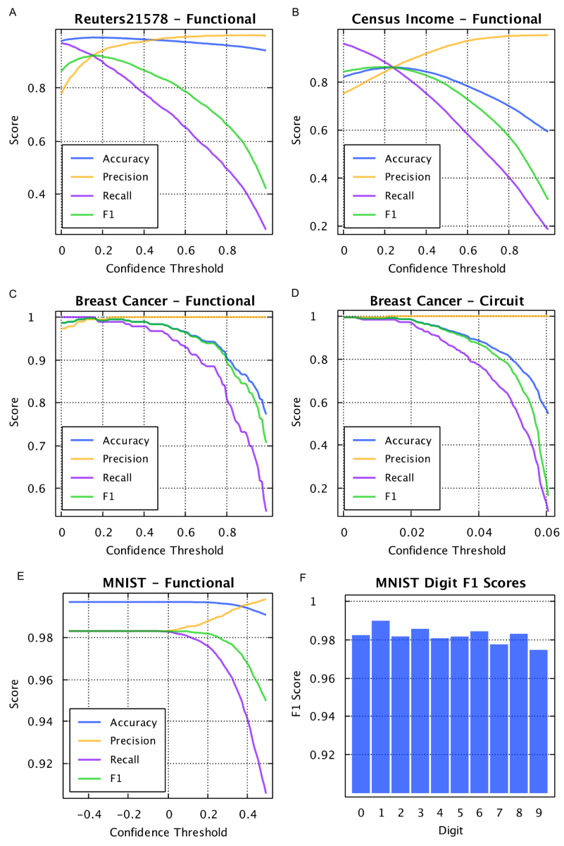
Fig. 16. Classification benchmarks results. A) Reuters-21578. Using the top ten most frequent labels associated with the news articles in the Reuters-21578 data set, the AHaH classifier’s accuracy, precision, recall, and F1 score was determined as a function of its confidence threshold. As the confidence threshold increases, the precision increases while recall drops. An optimal confidence threshold can be chosen depending on the desired results and can be dynamically changed. The peak F1 score is 0.92. B) Census Income. The peak F1 score is 0.86 C) Breast Cancer. The peak F1 score is 0.997. D) Breast Cancer repeated but using the circuit model rather than the functional model. The peak F1 score and the shape of the curves are similar to functional model results. E) MNIST. The peak F1 score is 0.98-.99, depending on the resolution of the spike encoding. F) The individual F1 classification scores of the hand written digits.

Complex signal prediction with the AHaH classifier

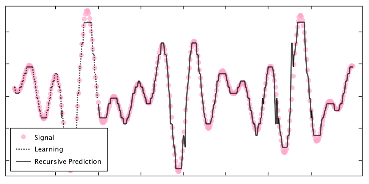
Fig. 18. Complex signal prediction with the AHaH classifier.} By posing prediction as a multi-label classification problem, the AHaH classifier can learn complex temporal waveforms and make extended predictions via recursion. Here, the temporal signal (dots) is a summation of five sinusoidal signals with randomly chosen amplitudes, periods, and phases. The classifier is trained for 10,000 time steps (last 100 steps shown, dotted line) and then tested for 300 time steps (solid line).

Select Videos